Page 183 - MATLAB an introduction with applications
P. 183

168 ———  MATLAB: An Introduction with Applications


                       ans =
                            –0.1282 + 2.6357i
                            –0.1282 – 2.6357i
                            –0.1436
                       >> % Nyquist plot
                       >> num =[0 0 0 1];
                       >> den =[1 0.4 7 1];
                       >> nyquist(num,den)
                       >> v=[–3 3 –2 2];axis(v);axis(‘square’)
                       >> grid
                       >> title(‘Nyquist plot of G(s)’)
                                                          Nyquist Diagram
                                 1

                                0.8

                                0.6

                                0.4
                              Imaginary Axis  0.2


                                 0

                                0.2

                                0.4

                                0.6

                                0.8

                                 1
                                  1    0.8   0.6   0.4   0.2   0     0.2  0.4   0.6   0.8   1
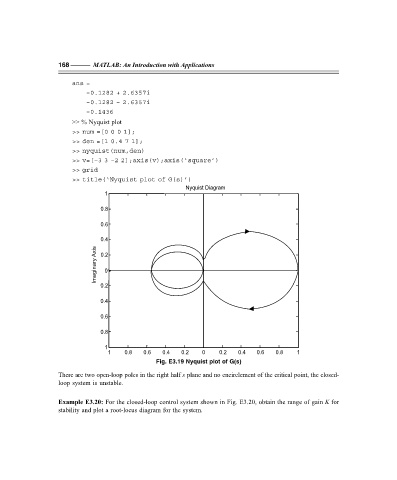
                                                 Fig. E3.19 Nyquist plot of G(s)

                   There are two open-loop poles in the right half s plane and no encirclement of the critical point, the closed-
                   loop system is unstable.


                   Example E3.20: For the closed-loop control system shown in Fig. E3.20, obtain the range of gain K for
                   stability and plot a root-locus diagram for the system.


                   F:\Final Book\Sanjay\IIIrd Printout\Dt. 10-03-09
   178   179   180   181   182   183   184   185   186   187   188