Page 186 - MATLAB an introduction with applications

Control Systems ——— 171

For this K value, we obtain the range of gain K for stability as
1.5894 > K > 0

Example E3.21: For the control system shown in Fig. E3.21:
(a) plot the root loci for the system
(b) find the value of K such that the damping ratio ζ of the dominant closed-loop poles is 0.6
(c) obtain all closed-loop poles
(d) plot the unit-step respond curve using MATLAB.

+ K
s ( s + 3 )( s + ) 5
–

Fig. E3.21
Solution:
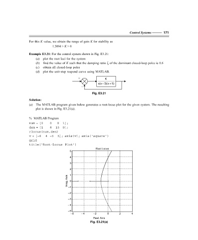
(a) The MATLAB program given below generates a root-locus plot for the given system. The resulting
plot is shown in Fig. E3.21(a).

% MATLAB Program
num = [0 0 0 1];
den = [1 8 15 0];
rlocus(num,den)
v = [–6 4 –5 5]; axis(v); axis(‘square’)
grid
title(‘Root-Locus Plot’)
Root Locus
5
4

3
2
Imag. Axis 1 x x x
0

–1
–2
–3

–4
–5
–6 – 4 –2 0 2 4
Real Axis
Fig. E3.21(a)

F:\Final Book\Sanjay\IIIrd Printout\Dt. 10-03-09