Page 191 - MATLAB an introduction with applications

176 ——— MATLAB: An Introduction with Applications

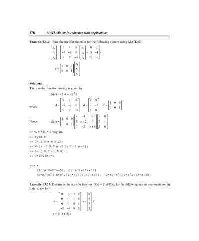
Example E3.24: Find the transfer function for the following system using MATLAB.


x

x   0 1 0   0 0 
1
1

 =− 5 − 2 0    3 − 1 u

+
x
x
     
2
2
x 


x
   0 2 − 6    5 0  
 
3
3
x 
1
 10 0 
y = x
  001  
2

x 

3
Solution:
The transfer function matrix is given by
()Gs = [ C sI − ] A − 1 B
 0 1 0  0  0  100

A =− 5 − 2 0  B =  3 − 1  C =   
where      001 
  0 2 − 6   5  0  
s  − 1 0   0 0 
 100    
Hence ()Gs =   5 s + 2 0 3 − 1
 001     

 0  − 2 s + 6 5  0  
 
>> % MATLAB Program
>> syms s
>> C=[1 0 0;0 0 1];
>> M=[s –1 0;5 s +2 0; 0 –2 s+6];
>> B=[0 0;3 –1;5 0];
>> C*inv(M)*B
ans =
[3/(s^2+2*s+5), –1/(s^2+2*s+5)]
[6*s/(s^3+8*s^2+17*s+30)+5/(s+6), –2*s/(s^3+8*s^2+17*s+30)]
Example E3.25: Determine the transfer function G(s) = Y(s)/R(s), for the following system representation in
state space form.
 0 3 7 0 0 
 0 0 1 0  
5

x =   x +  r
 0 0 0 1 7 
  
2 
−   5 − 6 9 5  
y = [1 3 6 5] x

F:\Final Book\Sanjay\IIIrd Printout\Dt. 10-03-09