Page 193 - MATLAB an introduction with applications

178 ——— MATLAB: An Introduction with Applications

0 

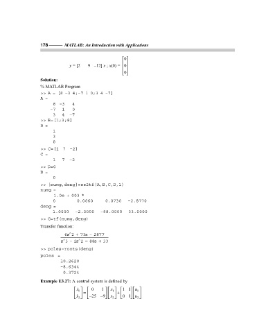
y = [2 9 –12] x ; x(0) = 0

0 

Solution:
% MATLAB Program

>> A = [8 –3 4;–7 1 0;3 4 –7]
A =
8–3 4
–7 1 0
3 4 –7
>> B=[1;3;8]
B =
1
3
8
>> C=[1 7 –2]
C =
1 7 –2
>> D=0
D =
0
>> [numg,deng]=ss2tf(A,B,C,D,1)
numg =
1.0e + 003 *
0 0.0060 0.0730 –2.8770
deng =
1.0000 –2.0000 –88.0000 33.0000
>> G=tf(numg,deng)
Transfer function:
∧
6s 2 + 73s – 2877
∧ ∧
s 3–2s 2 − 88s + 33
>> poles=roots(deng)
poles =
10.2620
–8.6344
0.3724
Example E3.27: A control system is defined by



x   0 1  x 1   1 1 u 

1
1
+
 =       
x
 
  − 25 − 9   x 2   0 1 u 2
2
F:\Final Book\Sanjay\IIIrd Printout\Dt. 10-03-09