
Page 192 - MATLAB an introduction with applications
P. 192
Control Systems ——— 177
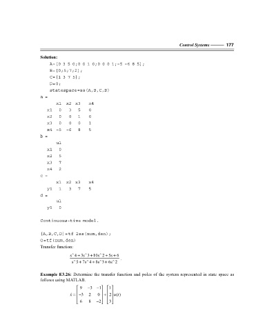
Solution:
A=[0 3 5 0;0 0 1 0;0 0 0 1;–5 –6 8 5];
B=[0;5;7;2];
C=[1 3 7 5];
D=0;
statespace=ss(A,B,C,D)
a =
x1 x2 x3 x4
x1 0 3 5 0
x2 0 0 1 0
x3 0 0 0 1
x4 –5 –6 8 5
b =
u1
x1 0
x2 5
x3 7
x4 2
c =
x1 x2 x3 x4
y1 1 3 7 5
d =
u1
y1 0
Continuous-time model.
[A,B,C,D]=tf 2ss(num,den);
G=tf(num,den)
Transfer function:
∧
∧
∧
+
+
+
+
s4 3s 3 10s2 5s 6 .
∧
∧
∧
∧
+
+
+
s5 7s 4 8s 3 6s 2
Example E3.26: Determine the transfer function and poles of the system represented in state space as
follows using MATLAB.
9 − 3 − 1
1
x =− 3 2 0 + 2 u ( )
t
6 8 − 2 3
F:\Final Book\Sanjay\IIIrd Printout\Dt. 10-03-09