Page 197 - MATLAB an introduction with applications

182 ——— MATLAB: An Introduction with Applications

>> C=[1 0];
>> D=[0];
>> % New enlarged state and output equations
>> AA=[A zeros (2, 1); C 0];
>> BB=[B; 0];
>> CC=[0 1];
>> DD=[0];
>> [z, x, t] =step (AA, BB, CC, DD);
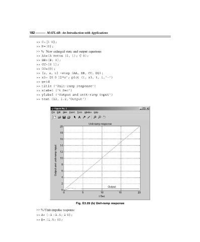
>> x3= [0 0 1]*x’; plot (t, x3, t, t,‘–’)
>> grid
>> title (‘Unit–ramp response’)
>> xlabel (‘t Sec’)
>> ylabel (‘Output and unit-ramp input’)
>> text (12, 1.2,‘Output’)

Unit-ramp response
20

18
16
input 14

12
unit-ramp 10

and 8
Output 6

4

2
Output
0
0 5 10 15 20
t Sec
Fig. E3.29 (b) Unit-ramp response
>> % Unit-impulse response

>> A= [–1 –1.5; 2 0];
>> B= [1.5; 0];

F:\Final Book\Sanjay\IIIrd Printout\Dt. 10-03-09