Page 201 - MATLAB an introduction with applications

186 ——— MATLAB: An Introduction with Applications

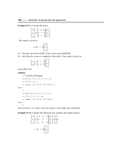
Example E3.31: Consider the system

 x   30 0   x 
 1     1 
x  2  =  01 0   x 2 
   032   x 
  x 3      3
The output is given by
x  1 

]
y = [11 1 x 
 2 
 x  3 
(a) determine the observability of the system using MATLAB
(b) show that the system is completely observable if the output is given by
x 
1
 y 1   11 1 
x
  =   
2
 y 2  13 2 
x 

3
using MATLAB.
Solution:
>> % MATLAB Program
>> A =[3 0 0; 0 1 0; 0 3 2];
>> C =[1 1 1];
>> rank ([C’ A’*C’ A’^2*C’])
ans=
3
>> A=[3 0 0; 0 1 0; 0 3 2];
>> C=[1 1 1; 1 3 2];
>> rank ([C’ A’*C’ A’^2*C’])
ans=
3
From the above, we observe that the system is observable and controllable.

Example E3.32: Consider the following state equation and output equation
2  

x  −  1 − 3 −  x 1 3
1
 =  0 − 2 1    
+
x
0 u
x
     
2
2
x 
1


x
   1 0 − 1    
 
3
3
x 
1

]
y = [11 0 x

2
x 

3
F:\Final Book\Sanjay\IIIrd Printout\Dt. 10-03-09