Page 206 - MATLAB an introduction with applications

Control Systems ——— 191

using MATLAB. Determine also the rise time, peak time, maximum overshoot and settling time in the unit-
step response plot.
P3.3: Obtain the unit-acceleration response curve of the unity-feedback control system whose open loop
transfer function is given by
8(s + 1)
() =
Gs
2
( +
ss 3)
using MATLAB. The unit-acceleration input is defined by
1
() =rt t 2 ( ≥ 0)
t
2
P3.4: The feed forward transfer function G(s) of a unity-feedback system is given by
( ks + 3) 2
() =
Gs
(s + 5)(s + 4) 2
2
Plot the root loci for the system using MATLAB.
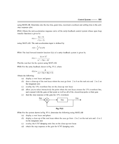
P3.5: For the unity feedback shown in Fig. P3.5, where
K
() =
Gs
( ss + 3)(s + 4)(s + 5)
Obtain the following:
(a) display a root locus and pause
(b) draw a close-up of the root locus where the axes go from –2 to 0 on the real axis and –2 to 2 on
the imaginary axis
(c) overlay the 15% overshoot line on the close-up root locus
(d) allow you to select interactively the point where the root locus crosses the 15% overshoot line,
and respond with the gain at that point as well as all of the closed-loop poles at that gain
(e) find the step response at the gain for 15% overshoot.

R(s) + C(s)
G(s)
–

Fig. P3.5

P3.6: For the system shown in Fig. P3.6, determine the following using MATLAB
(a) display a root locus and phase
(b) display a close-up of the root locus where the axes go from –2 to 2 on the real axis and –2 to 2
on the imaginary axis
(c) overlay the 0.707 damping ratio line on the close-up root locus
(d) obtain the step response at the gain for 0.707 damping ratio.

F:\Final Book\Sanjay\IIIrd Printout\Dt. 10-03-09