Page 209 - MATLAB an introduction with applications

194 ——— MATLAB: An Introduction with Applications

P3.15: For a unit feedback system with the forward-path transfer function

K
() =
Gs
( ss + 3)(s + 10)
and a delay of 0.5 second, estimate the percent overshoot for K = 40 using a second-order approximation.
Model the delay using MATLAB function pade(T, n). Determine the unit step response and check the
second-order approximation assumption made.

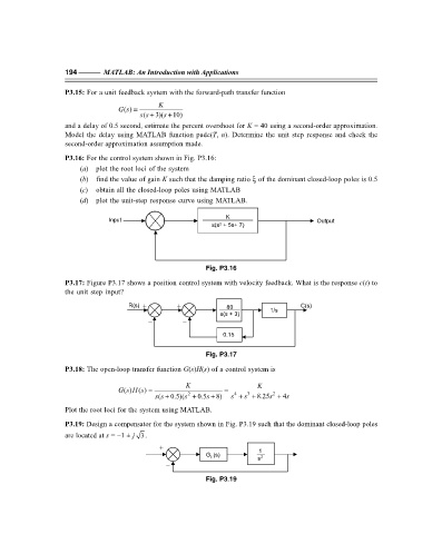
P3.16: For the control system shown in Fig. P3.16:
(a) plot the root loci of the system
(b) find the value of gain K such that the damping ratio ξ of the dominant closed-loop poles is 0.5
(c) obtain all the closed-loop poles using MATLAB
(d) plot the unit-step response curve using MATLAB.

K
Input Output
2
s(s + 5s+ 7)

Fig. P3.16
P3.17: Figure P3.17 shows a position control system with velocity feedback. What is the response c(t) to
the unit step input?

R(s) + + 80 C(s)
1/s
s(s+3)
– –
0.15

Fig. P3.17
P3.18: The open-loop transfer function G(s)H(s) of a control system is

K K
() ( ) s =
Gs H =
3
4
2
2
( ss + 0.5)(s + 0.5s + 8) s + s + 8.25s + 4s
Plot the root loci for the system using MATLAB.
P3.19: Design a compensator for the system shown in Fig. P3.19 such that the dominant closed-loop poles
are located at s = –1 ± j 3.
+ 1
G c (s)
s 2
–

Fig. P3.19

F:\Final Book\Sanjay\IIIrd Printout\Dt. 10-03-09