Page 208 - MATLAB an introduction with applications

Control Systems ——— 193

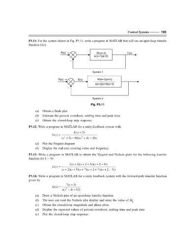
P3.11: For the system shown in Fig. P3.11, write a program in MATLAB that will use an open-loop transfer
function G(s).

R(s) + 80 s ( + ) 2 C(s)
s ( s + s ( ) 1 + ) 3
–

System 1

R(s) + E(s) 40(s+3)(s+5)
s(s+2)(s+4)(s+6)
–

System 2

Fig. P3.11
(a) Obtain a Bode plot
(b) Estimate the percent overshoot, settling time and peak time
(c) Obtain the closed-loop step response.
P3.12: Write a program in MATLAB for a unity-feedback system with
( +
Ks 3)
() =
Gs
2
(s + 5s + 80)(s + 4s + 20)
2
(a) Plot the Nyquist diagram
(b) Display the real-axis crossing value and frequency.
P3.13: Write a program in MATLAB to obtain the Nyquist and Nichols plots for the following transfer
function for k = 30.

2 5 )(s + −
( k s + 1)(s + + i 2 5 )
i
() =
Gs
(s + 2)(s + 5)(s + 7)(s + + i 2 7 )
2 7 )(s + −
i
P3.14: Write a program in MATLAB for a unity feedback system with the forward-path transfer function
given by
7(s + 3)
() =
Gs
2
( ss + 4s + 12)
(a) Draw a Nichols plot of an open-loop transfer function
(b) The user can read the Nichols plot display and enter the value of M p
(c) Obtain the closed-loop magnitude and phase plots.
(d) Display the expected values of percent overshoot, settling time and peak time
(e) Plot the closed-loop step response.

F:\Final Book\Sanjay\IIIrd Printout\Dt. 10-03-09