Page 211 - MATLAB an introduction with applications

196 ——— MATLAB: An Introduction with Applications

x 
1

y = [0 25 5] x 2 + [0]u

x 

3
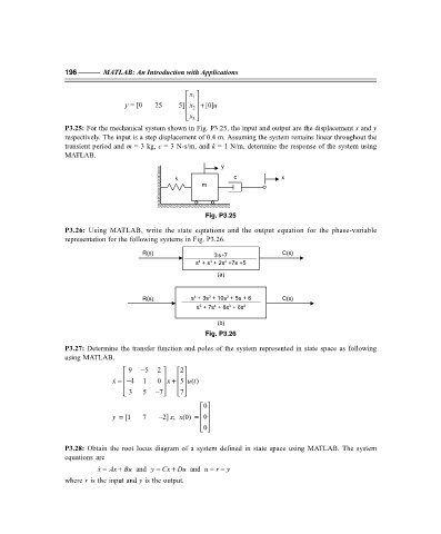
P3.25: For the mechanical system shown in Fig. P3.25, the input and output are the displacement x and y
respectively. The input is a step displacement of 0.4 m. Assuming the system remains linear throughout the
transient period and m = 3 kg, c = 3 N-s/m, and k = 1 N/m, determine the response of the system using
MATLAB.
y
k c x
m

Fig. P3.25
P3.26: Using MATLAB, write the state equations and the output equation for the phase-variable
representation for the following systems in Fig. P3.26.

R(s) C(s)
3+ 7
s
4
3
2
s + s + 2s +7s +5
(a)
2
3
4
R(s) s +3s +10s +5s+6 C(s)
5
3
4
s+ 7s+ 8s+ 6s 2
(b)
Fig. P3.26
P3.27: Determine the transfer function and poles of the system represented in state space as following
using MATLAB.
 9 − 5 2  2  


x =− 4 1 0 x +   ( )

5 u
t

 

7  
  3 5 − 7   
0 
0
y = [1 7 –2] x; x(0) = 

0 

P3.28: Obtain the root locus diagram of a system defined in state space using MATLAB. The system
equations are
x = Ax Bu and y = Cx Du and u = − y
+
+

r
where r is the input and y is the output.

F:\Final Book\Sanjay\IIIrd Printout\Dt. 10-03-09