Page 210 - MATLAB an introduction with applications

Control Systems ——— 195

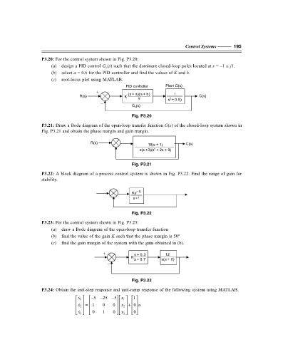
P3.20: For the control system shown in Fig. P3.20:
(a) design a PID control G (s) such that the dominant closed-loop poles located at s = –1 ± j1.
c
(b) select a = 0.6 for the PID controller and find the values of K and b.
(c) root-locus plot using MATLAB.
PID controller Plant G(s)
+
R(s) K s ( + a )( s + ) b 1 C(s)
s s + ) 8 . 0
2
–
G c (s)
Fig. P3.20
P3.21: Draw a Bode diagram of the open-loop transfer function G(s) of the closed-loop system shown in
Fig. P3.21 and obtain the phase margin and gain margin.

R(s) C(s)
18(s + 1)
s(s +3)(s + 2s + 9)
2

Fig. P3.21
P3.22: A block diagram of a process control system is shown in Fig. P3.22. Find the range of gain for
stability.

Ke s
s+ 1

Fig. P3.22
P3.23: For the control system shown in Fig. P3.23:
(a) draw a Bode diagram of the open-loop transfer function
(b) find the value of the gain K such that the phase margin is 50º
(c) find the gain margin of the system with the gain obtained in (b).

+ s + 3 . 0 12
K
s + 7 . 0 s ( s + ) 2
–

Fig. P3.23

P3.24: Obtain the unit-step response and unit-ramp response of the following system using MATLAB.

x  −  5 − 25 −  1 1
5 x   
1
 =  1 0 0    
x
+
x
0 u
     
2
2
0

x 
x

   0 1 0    
 
3
3
F:\Final Book\Sanjay\IIIrd Printout\Dt. 10-03-09