Page 94 - MATLAB Recipes for Earth Sciences

5.2 Generating Signals 87

samples equally spaced along the sediment core are therefore not equally
spaced on the time axis. In this case, the quantity

where T is the full length of the time series and N is the number of data points,
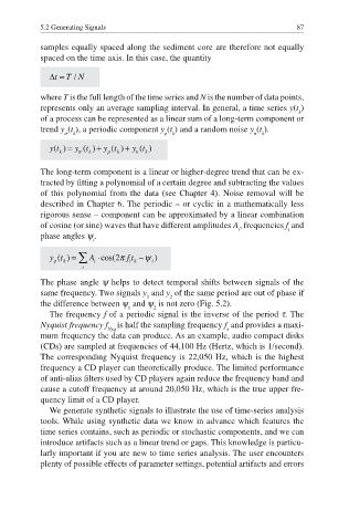
represents only an average sampling interval. In general, a time series y(t )
k
of a process can be represented as a linear sum of a long-term component or
trend y (t ), a periodic component y (t ) and a random noise y (t ).
tr k p k n k

The long-term component is a linear or higher-degree trend that can be ex-

tracted by fitting a polynomial of a certain degree and subtracting the values
of this polynomial from the data (see Chapter 4). Noise removal will be
described in Chapter 6. The periodic – or cyclic in a mathematically less
rigorous sense – component can be approximated by a linear combination
of cosine (or sine) waves that have different amplitudes A , frequencies f and
i i
phase angles ψ .
i

The phase angle ψ helps to detect temporal shifts between signals of the
same frequency. Two signals y and y of the same period are out of phase if
1 2
the difference between ψ and ψ is not zero (Fig. 5.2).
1 2
The frequency f of a periodic signal is the inverse of the period τ. The
Nyquist frequency f is half the sampling frequency f and provides a maxi-
Nyq s
mum frequency the data can produce. As an example, audio compact disks
(CDs) are sampled at frequencies of 44,100 Hz (Hertz, which is 1/second).
The corresponding Nyquist frequency is 22,050 Hz, which is the highest
frequency a CD player can theoretically produce. The limited performance

of anti-alias filters used by CD players again reduce the frequency band and
cause a cutoff frequency at around 20,050 Hz, which is the true upper fre-
quency limit of a CD player.
We generate synthetic signals to illustrate the use of time-series analysis
tools. While using synthetic data we know in advance which features the
time series contains, such as periodic or stochastic components, and we can
introduce artifacts such as a linear trend or gaps. This knowledge is particu-
larly important if you are new to time series analysis. The user encounters
plenty of possible effects of parameter settings, potential artifacts and errors