Page 98 - MATLAB Recipes for Earth Sciences

5.3 Autospectral Analysis 91

Such trends are common features in earth sciences. As an example, consider
the glacial-interglacial cycles observed in marine oxygen isotope records
overlain by a long-term cooling trend during the last six million years.

yt = y + 0.005 * t;
plot(t,y,'b-',t,yt,'r-'), axis([0 200 -4 4])
In reality, more complex trends exist, such as higher-order trends or trends
characterized by changing slopes. In practice, it is recommended to elimi-

nate such a trend by fitting polynomials to the data and to subtract the the
corresponding values. This synthetic time series now contains many charac-
teristics of a typical data set in the earth sciences. It can be used to illustrate
the use of spectral analysis tools that are introduced in the next chapter.

5.3 Autospectral Analysis

Autospectral analysis aims to describe the distribution of variance contained
in one single signal x(t) over frequency or wavelength. A simple way to
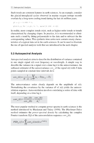
describe the variance in a signal over a time lag k is the autocovariance. An
unbiased estimator of the autocovariance cov of the signal x(t) with N data
xx
points sampled at constant time intervals ¨t is

The autocovariance series clearly depends on the amplitude of x(t).
2
Normalizing the covariance by the variance σ of x(t) yields the autocor-
relation sequence. Autocorrelation involves correlating a series of data with
itself, depending on a time lag k.

The most popular method to compute power spectra in earth sciences is the
method introduced by Blackman and Tukey (1958). The Blackman-Tukey
method estimates the power-spectral density by calculating the complex
Fourier transform X(f) of the autocorrelation sequence corr (k).
xx