Page 103 - MATLAB Recipes for Earth Sciences

96 5 Time-Series Analysis

Power Spectral Power Spectral
Density Estimate Density Estimate
1000 7000
6000 Linear trend
800 f 1 =0.02
5000
Power 600 f 2 =0.07 Power 4000

400 3000
2000 f 1 =0.02
f 3 =0.2
200 f 2 =0.07
1000 f 3 =0.2
0 0
0 0.1 0.2 0.3 0.4 0.5 0 0.1 0.2 0.3 0.4 0.5
Frequency Frequency
a b
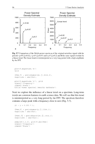
Fig. 5.7 Comparison of the Welch power spectra a of the original noisefree signal with the
periods τ =50 (f =0.02), τ =15 (f §0.07) and τ =5 (f =0.2) and b the same signal overlain by
1 1 2 2 3 3
a linear trend. The linear trend is misinterpreted as a very long period with a high amplitude
by the FFT.

plot(f,magnitude,'b')
hold
[Pxx,f] = periodogram(yn,[],1024,1);
magnitude = abs(Pxx);

plot(f,magnitude,'r'), grid
xlabel('Frequency')
ylabel('Power')
title('Power Spectral Density Estimate')

Next we explore the influence of a linear trend on a spectrum. Long-term
trends are common features in earth science data. We will see that this trend
is misinterpreted as a very long period by the FFT. The spectrum therefore
contains a large peak with a frequency close to zero (Fig. 5.7).
yt = y + 0.005 * t;

[Pxx,f] = periodogram(y,[],1024,1);
magnitude = abs(Pxx);
[Pxxt,f] = periodogram(yt,[],1024,1);
magnitudet = abs(Pxxt);
subplot(1,2,1), plot(f,abs(Pxx))
xlabel('Frequency')
ylabel('Power')