Page 104 - MATLAB Recipes for Earth Sciences

5.4 Crossspectral Analysis 97

subplot(1,2,2), plot(f,abs(Pxxt))
xlabel('Frequency')
ylabel('Power')

To eliminate the long-term trend, we use the function detrend.

ydt = detrend(yt);
subplot(2,1,1)
plot(t,y,'b-',t,yt,'r-'), axis([0 200 -4 4])

subplot(2,1,2)
plot(t,y,'b-',t,ydt,'r-'), axis([0 200 -4 4])
The corresponding spectrum does not show the low-frequency peak any-
more. Some data contain a high-order trend that can be removed by fi tting
a higher-order polynomial to the data and by subtracting the corresponding
x(t) values.

5.4 Crossspectral Analysis

Crossspectral analysis correlates two time series in the frequency domain.
The crosscovariance is as a measure for the variance in two signals over a
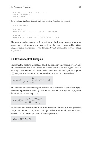
time lag k. An unbiased estimator of the crosscovariance cov of two signals
xy
x(t) and y(t) with N data points sampled at constant time intervals ¨t is

The crosscovariance series again depends on the amplitudes of x(t) and y(t).
Normalizing the covariance by the standard deviations of x(t) and y(t) yields
the crosscorrelation sequence.

In practice, the same methods and modifications outlined in the previous
chapter are used to compute the crossspectral density. In addition to the two
autospectra of x(t) and y(t) and the crossspectrum,