Page 54 - MEMS Mechanical Sensors

3.2 Simulation and Design Tools 43

PID controller
Output
−
8.2e 6 1.22e5 10e 6 −1.59e6
−
signal
1
1.0 1.0 −6
−
0v 0 1 + .3888e-3vs+72.9e 9vs*s
1/seismic 1 −10e −6 Gain of the Lowpass filter
0.5 mass Nonlinear
pick-off circuit −0.6
damping 2
VOCC 0
d
dt 0
0
12.3
83.3 Bias voltage
Parameters: 50
freq 0.5 Spring constant 1
1
2
2 −12.3
El.-st force generated −15 Bias voltage
by voltage on bottom plate
1 −50
2
15
El.-st force generated Saturation of drive amplifiers
by voltage on top plate
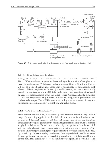
Figure 3.3 System level model of a closed loop micromachined accelerometer in Orcad PSpice.

3.2.1.3 Other System Level Simulators
A range of other system level simulators exists which are suitable for MEMS. Vis-
Sim is a Windows-based program for the modeling and simulation of complex non-
linear dynamic systems [7]. It is very similar in its capabilities to Simulink and hence
will not be reviewed further here. Saber from Synopsis software simulates physical
effects in different engineering domains (hydraulic, electric, electronic, mechanical)
as well as signal-flow algorithms [8]. Saber is designed to perform simulations based
on very few preconceptions about the target system. Consequently, the simulator
can analyze designs containing multiple technologies, using the analysis units native
to these technologies. The MEMS-relevant technologies include: electronic, electro-
mechanical, mechanical, electro-optical, and controls systems.

3.2.2 Finite Element Simulation Tools

Finite element analysis (FEA) is a commonly used approach for simulating a broad
range of engineering applications. The finite element method is well suited to the
solution of differential equations with known boundary conditions, and it enables
the analysis of complex geometries by subdividing them into a finite number of more
simply shaped elements. Each element is defined by nodal points and can be specified
with particular characteristics relevant to the engineering problem being solved. The
solution involves approximating the required function over each finite element and,
by considering element boundary conditions, obtaining nodal values of the function
for each particular element. After considering interelement equilibrium and known
global boundary conditions, a set of simultaneous equations is obtained. The