Page 51 - MEMS Mechanical Sensors

40 MEMS Simulation and Design Tools

successfully applied to simulate electromagnetic fields, thermodynamic prob-
lems such as squeeze film damping, and fluidics. FEM results in more realistic
simulation results than behavioral modeling, but it is much more computa-
tionally demanding and hence it is difficult to simulate entire systems.

3.2 Simulation and Design Tools

3.2.1 Behavioral Modeling Simulation Tools
3.2.1.1 Matlab and Simulink

One of the most popular behavioral modeling tools is Simulink, which is a toolbox
within Matlab [1]. It allows the user to perform system level simulation in the time
domain. The user chooses blocks from a library that includes linear and nonlinear
functions, which are either time continuous or discrete. Examples include gain, inte-
grators and differentiators, z- and s-domain transfer functions, limiters, samplers,
mathematical functions, switches, and many others.
Each block has a range of input and outputs. An input can be the output of
another block or a source that can be an arbitrary waveform. Any output of a block
can be visualized by different types of plots in the time or frequency domain; alterna-
tively it can be stored as a variable to be analyzed or filtered further in Matlab. The
software allows user-defined library and hierarchal modeling by defining parame-
terized subsystems. The software has a purely graphical interface; blocks are chosen
by drag and drop and connected by wires drawn on the screen.
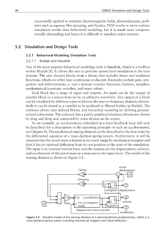
As an example, an accelerometer embedded in a force-feedback loop will now
be described (for a description of the operating principle of such an accelerometer,
see Chapter 8). The mechanical sensing element can be described to the first order by
the differential equation of a mass-dashpot-spring system. Furthermore, it will be
assumed that the proof mass is limited in its travel range by mechanical stoppers and
that it has an optional deflection from its rest position at the start of the simulation.
The input is an external inertial force and the outputs are the displacement, velocity,
and acceleration of the proof mass as a response to the input force. The model of the
sensing element is shown in Figure 3.1.

at-rest
Spring displacement
k x0
Damping
b 1
s 1
x o
x
Integrator displacement
− 1/m F/m a acceleration 2
− 1 v
1 + Mass x Int_res integrator s velocity
Fext result Integrator1
3
Displacement limit controller a
acceleration
Figure 3.1 Simulink model of the sensing element of a micromachined accelerometer, which is a
mass-dashpot-spring system including mechanical stoppers and initial deflection.