Page 159 - Macromolecular Crystallography

148 MACROMOLECULAR CRYS TALLOGRAPHY

(a) probability distributions: (1) real space restraints
give distributions for modified structure factors,
while (2) the phasing experiments give partially
independent phase probability distributions. Com-
bining distributions is easy: we just multiply them,
provided we know they are independent. However,
here consecutive distributions are clearly not inde-
pendent and treating them as independent would
inevitably lead to an undesirable bias towards the
(b)
very first map with which we started the Fourier
cycling. How do we deal with this situation? We
separate out the dependent component, and multiply
the independent components. In order to explain
how this is done in practice, we give a more
quantitative explanation of the reason why Fourier
cycling and phase recombination works, first for
solvent flattening and subsequently for NCS and
(c) histogram matching.

10.7 Why does Fourier cycling improve
phases in solvent flattening?
Before we can flatten the solvent, we need to know
where it is. One of the implementations to obtain a
good approximation of the solvent mask computes
the variance of the electron density within a small
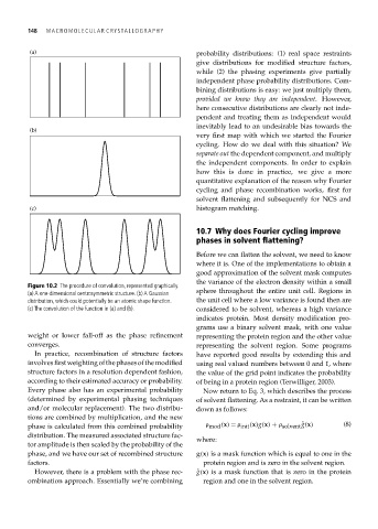
Figure 10.2 The procedure of convolution, represented graphically.
(a) A one-dimensional centrosymmetric structure. (b) A Gaussian sphere throughout the entire unit cell. Regions in
distribution, which could potentially be an atomic shape function. the unit cell where a low variance is found then are
(c) The convolution of the function in (a) and (b). considered to be solvent, whereas a high variance
indicates protein. Most density modification pro-
grams use a binary solvent mask, with one value
weight or lower fall-off as the phase refinement representing the protein region and the other value
converges. representing the solvent region. Some programs
In practice, recombination of structure factors have reported good results by extending this and
involvesfirstweightingofthephasesofthemodified using real valued numbers between 0 and 1, where
structure factors in a resolution dependent fashion, the value of the grid point indicates the probability
according to their estimated accuracy or probability. of being in a protein region (Terwilliger, 2003).
Every phase also has an experimental probability Now return to Eq. 3, which describes the process
(determined by experimental phasing techniques of solvent flattening. As a restraint, it can be written
and/or molecular replacement). The two distribu- down as follows:
tions are combined by multiplication, and the new
phase is calculated from this combined probability ρ mod (x) = ρ init (x)g(x) + ρ solvent ˆ g(x) (8)
distribution. The measured associated structure fac-
where:
tor amplitude is then scaled by the probability of the
phase, and we have our set of recombined structure g(x) is a mask function which is equal to one in the
factors. protein region and is zero in the solvent region.
However, there is a problem with the phase rec- ˆ g(x) is a mask function that is zero in the protein
ombination approach. Essentially we’re combining region and one in the solvent region.