Page 124 - Mathematical Models and Algorithms for Power System Optimization

114 Chapter 4

4.8.2 Conditions and Results of Four Cases for 135-Bus Large-scale System

This case study uses a real-scale 135-node test system that consists of 36 generators, 98 loads,
and 17 transformers. The mathematical programming system (MPS) is used for solving LP
problems. Calculation results for the four cases shown in Tables 4.16–4.18 are given to
demonstrate the performance of the algorithm. The initial points of cases 1 and 3 are the results
of continuous OPF solutions obtained by the nonlinear method MINOS/AUGMENTED
Ver. 4.0 [22].

Because the discrete OPF is a nonconvex problem, the optimal solution obtained by the SLP
technique is related to the initial value. To demonstrate the effectiveness of the algorithm
proposed in this chapter, four cases are studied. The initial values in case 1 and case 3 utilize the
optimal solutions of continuous OPF obtained by the nonlinear method of MINOS/
AUGMENTED Ver. 4.0. The algorithm proposed requires an initial integer solution, thus, the
integer variables of the optimal solution to the continuous OPF is rounded off to form the initial
integer solution. In comparison, the initial values of case 2 and case 4 utilize the conventional
power flow solutions under the normal operation condition. In addition, the initial values of
cases 1–4 are continuously feasible, whereas the rounded values are infeasible, which validates
the effectiveness of the algorithm.

In these numerical cases, to distinguish the local optimal solutions, a big difference for the
generation cost is assigned according to the characteristics of the generators. The resulting
difference value of the objective function between the optimal operation state and the general
one is about 10%. The voltage magnitude is allowed a variation of ranges with 0.94–1.06 for
case 1 and case 2, and 0.97–1.03 for case 3 and case 4.

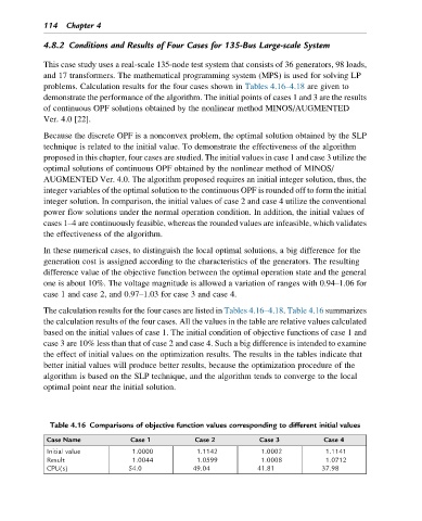
The calculation results for the four cases are listed in Tables 4.16–4.18. Table 4.16 summarizes
the calculation results of the four cases. All the values in the table are relative values calculated
based on the initial values of case 1. The initial condition of objective functions of case 1 and
case 3 are 10% less than that of case 2 and case 4. Such a big difference is intended to examine
the effect of initial values on the optimization results. The results in the tables indicate that
better initial values will produce better results, because the optimization procedure of the
algorithm is based on the SLP technique, and the algorithm tends to converge to the local
optimal point near the initial solution.

Table 4.16 Comparisons of objective function values corresponding to different initial values

Case Name Case 1 Case 2 Case 3 Case 4
Initial value 1.0000 1.1142 1.0002 1.1141
Result 1.0044 1.0599 1.0008 1.0712
CPU(s) 54.0 49.04 41.81 37.98