Page 125 - Mathematical Models and Algorithms for Power System Optimization

New Algorithms Related to Power Flow 115

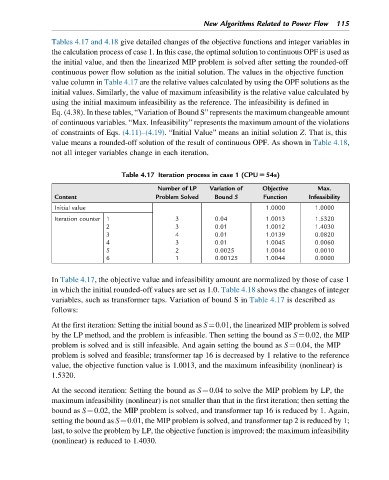
Tables 4.17 and 4.18 give detailed changes of the objective functions and integer variables in
the calculation process of case 1. In this case, the optimal solution to continuous OPF is used as
the initial value, and then the linearized MIP problem is solved after setting the rounded-off
continuous power flow solution as the initial solution. The values in the objective function
value column in Table 4.17 are the relative values calculated by using the OPF solutions as the
initial values. Similarly, the value of maximum infeasibility is the relative value calculated by
using the initial maximum infeasibility as the reference. The infeasibility is defined in
Eq. (4.38). In these tables, “Variation of Bound S” represents the maximum changeable amount
of continuous variables. “Max. Infeasibility” represents the maximum amount of the violations
of constraints of Eqs. (4.11)–(4.19). “Initial Value” means an initial solution Z. That is, this
value means a rounded-off solution of the result of continuous OPF. As shown in Table 4.18,
not all integer variables change in each iteration.

Table 4.17 Iteration process in case 1 (CPU554s)
Number of LP Variation of Objective Max.
Content Problem Solved Bound S Function Infeasibility
Initial value 1.0000 1.0000
Iteration counter 1 3 0.04 1.0013 1.5320
2 3 0.01 1.0012 1.4030
3 4 0.01 1.0139 0.0820
4 3 0.01 1.0045 0.0060
5 2 0.0025 1.0044 0.0010
6 1 0.00125 1.0044 0.0000

In Table 4.17, the objective value and infeasibility amount are normalized by those of case 1
in which the initial rounded-off values are set as 1.0. Table 4.18 shows the changes of integer
variables, such as transformer taps. Variation of bound S in Table 4.17 is described as
follows:

At the first iteration: Setting the initial bound as S¼0.01, the linearized MIP problem is solved
by the LP method, and the problem is infeasible. Then setting the bound as S¼0.02, the MIP
problem is solved and is still infeasible. And again setting the bound as S¼0.04, the MIP
problem is solved and feasible; transformer tap 16 is decreased by 1 relative to the reference
value, the objective function value is 1.0013, and the maximum infeasibility (nonlinear) is
1.5320.

At the second iteration: Setting the bound as S¼0.04 to solve the MIP problem by LP, the
maximum infeasibility (nonlinear) is not smaller than that in the first iteration; then setting the
bound as S¼0.02, the MIP problem is solved, and transformer tap 16 is reduced by 1. Again,
setting the bound as S¼0.01, the MIP problem is solved, and transformer tap 2 is reduced by 1;
last, to solve the problem by LP, the objective function is improved; the maximum infeasibility
(nonlinear) is reduced to 1.4030.