Page 212 - Mathematical Models and Algorithms for Power System Optimization

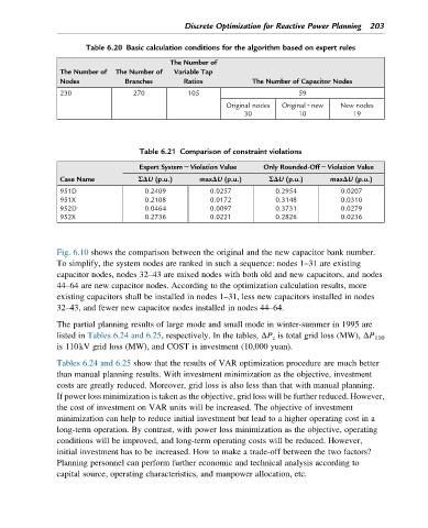
Discrete Optimization for Reactive Power Planning 203

Table 6.20 Basic calculation conditions for the algorithm based on expert rules
The Number of
The Number of The Number of Variable Tap
Nodes Branches Ratios The Number of Capacitor Nodes

230 270 105 59
Original nodes Original+new New nodes
30 10 19

Table 6.21 Comparison of constraint violations

Expert System2Violation Value Only Rounded-Off2Violation Value
Case Name ΣΔU (p.u.) maxΔU (p.u.) ΣΔU (p.u.) maxΔU (p.u.)
951D 0.2409 0.0257 0.2954 0.0207
951X 0.2108 0.0172 0.3148 0.0310
952D 0.0464 0.0097 0.3731 0.0279
952X 0.2736 0.0221 0.2826 0.0236

Fig. 6.10 shows the comparison between the original and the new capacitor bank number.
To simplify, the system nodes are ranked in such a sequence: nodes 1–31 are existing
capacitor nodes, nodes 32–43 are mixed nodes with both old and new capacitors, and nodes
44–64 are new capacitor nodes. According to the optimization calculation results, more
existing capacitors shall be installed in nodes 1–31, less new capacitors installed in nodes
32–43, and fewer new capacitor nodes installed in nodes 44–64.
The partial planning results of large mode and small mode in winter-summer in 1995 are

listed in Tables 6.24 and 6.25, respectively. In the tables, ΔP z is total grid loss (MW), ΔP 110
is 110kV grid loss (MW), and COST is investment (10,000 yuan).

Tables 6.24 and 6.25 show that the results of VAR optimization procedure are much better
than manual planning results. With investment minimization as the objective, investment
costs are greatly reduced. Moreover, grid loss is also less than that with manual planning.
If power loss minimization is taken as the objective, grid loss will be further reduced. However,
the cost of investment on VAR units will be increased. The objective of investment
minimization can help to reduce initial investment but lead to a higher operating cost in a
long-term operation. By contrast, with power loss minimization as the objective, operating
conditions will be improved, and long-term operating costs will be reduced. However,
initial investment has to be increased. How to make a trade-off between the two factors?
Planning personnel can perform further economic and technical analysis according to
capital source, operating characteristics, and manpower allocation, etc.