Page 272 - Mathematical Models and Algorithms for Power System Optimization

264 Chapter 7

_
X ¼ AX + Bu
_
Y ¼ CX + Du
The coefficients A and B are finalized by simultaneously uniting all first-order differential
equations, the coefficient of equations C and D are:

C ¼ 0, 0, …,1Š, D ¼ 0
½
provided the system output is X n .

2. If the system’s differential equation is known, its difference equation can be solved using
the following equation:

ϕτðÞ ¼ e Aτ
ð τ (7.117)
AT
ϕτðÞ ¼ e dT B
0
Consequently:

ð
Xk +1Þ ¼ ϕτðÞXkðÞ + G τðÞukðÞ
Step 2: Normalizing the difference equation. The state equation and transfer function of a
system are correlated by the normalization of state equation. The coefficients of the
normalized equation reflect those of the transfer function. Therefore, the state equation
must be normalized to obtain the system’s transfer function.
The dynamic system has been given as follows:
ð
Xk +1Þ ¼ ϕXkðÞ + Gu kðÞ
(7.118)
T T
½
ZkðÞ ¼ h XkðÞ,h ¼ h 1 , h 2 , …, h n Š
1 n
which can be transformed into:
∗
ð
Yk +1Þ ¼ ϕ YkðÞ + G ∗ ukðÞ
(7.119)
T
ZkðÞ ¼ h ∗ YkðÞ
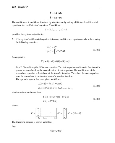
where

The transform process is shown as follows

Let:

YkðÞ ¼ FX kðÞ