Page 275 - Mathematical Models and Algorithms for Power System Optimization

Optimization Method for Load Frequency Feed Forward Control 267

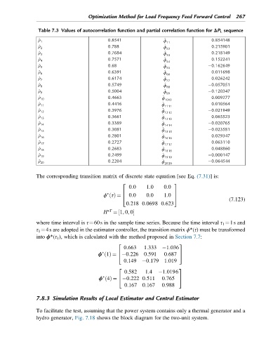
Table 7.3 Values of autocorrelation function and partial correlation function for ΔP L sequence
^ ρ ϕ
^
1 0.8541 0.854148
11
^
^ ρ ϕ
2 0.788 0.215901
22
^ ρ ϕ
^
3 0.7684 0.218149
33
^
^ ρ ϕ
4 0.7571 0.152241
44
^
^ ρ ϕ
5 0.68 0.162649
55
^ ρ ϕ
^
6 0.6391 0.011698
66
^
^ ρ ϕ
7 0.6174 0.026242
77
^ ρ ϕ
^
8 0.5749 0.057051
88
^
^ ρ ϕ
0.5004 0.120347
9
99
^ ρ ^
ϕ
10 0.4663 0.009277
1010
^ ρ ϕ
^
11 0.4416 0.010564
1111
^
^ ρ ϕ
12 0.3976 0.021949
1212
^ ρ ϕ
^
13 0.3661 0.065523
1313
^
^ ρ 0.3389 ϕ 0.020765
14
1414
^ ρ ϕ
^
15 0.3081 0.023581
1515
^ ρ ϕ
^
16 0.2801 0.029347
1616
^ ρ ϕ
^
17 0.2727 0.063110
1717
^ ρ ϕ
^
18 0.2683 0.048860
1818
^
^ ρ ϕ
19 0.2499 0.000147
1919
^ ρ ϕ
^
20 0.2204 0.064544
2020
The corresponding transition matrix of discrete state equation [see Eq. (7.31)] is:
2 3
0:0 1:0 0:0
∗ 6 0:0 0:0 7
(7.123)
ϕ τðÞ ¼ 4 1:0 5
0:218 0:0698 0:623
T
H ∗ ¼ 1, 0, 0½ Š
where time interval is τ¼60s in the sample time series. Because the time interval τ 1 ¼1s and
τ 1 ¼4s are adopted in the estimator controller, the transition matrix ϕ∗(τ) must be transformed
into ϕ∗(τ 1 ), which is calculated with the method proposed in Section 7.7:
2 3
0:663 1:333 1:036
∗
ϕ 1ðÞ ¼ 0:226 0:591 0:687 5
4
0:149 0:179 1:019
2 3
0:582 1:4 1:0196
∗
ϕ 4ðÞ ¼ 0:222 0:511 0:765 5
4
0:167 0:167 0:988
7.8.3 Simulation Results of Local Estimator and Central Estimator
To facilitate the test, assuming that the power system contains only a thermal generator and a
hydro generator, Fig. 7.18 shows the block diagram for the two-unit system.