Page 299 - Mathematical Techniques of Fractional Order Systems

288 Mathematical Techniques of Fractional Order Systems

Then consider the following Lorenz system (Sun et al., 2016):
α
D y 1 5 b 1 ðy 2 2 y 1 Þ 1 u 1
α
D y 2 5 b 2 y 1 2 y 2 2 y 1 y 3 1 u 2 ð10:4Þ
α
D y 3 52 b 3 y 3 1 1 ðy y 2 1 y 1 y Þ 1 u 3
1
2
2
where y i 5 y ri 1 y iim j, y i AC for i 5 1; 2, y i 5 y ri , y i AR for i 5 3 , and finally y i
is the complex conjugate. The input variables are u i 5 u ri 1 u iim j, u i AC for
i 5 1; 2, u i 5 u ri , u i AR for i 5 3. In order to set the system in chaotic regime
the constant values must be b 1 5 10, b 2 5 180, and b 3 5 1 with the initial
T
condition yð0Þ 5 ½0:110:1j; 0:110:1j; 0:1Š and α 5 0:95 so the following
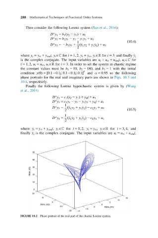
phase portraits for the real and imaginary parts are shown in Figs. 10.3 and
10.4, respectively.
Finally the following Lorenz hyperchaotic system is given by (Wang
et al., 2014)
α
D y 1 5 c 1 ðy 2 2 y 1 Þ 1 y 4 j 1 u 1
α
D y 2 5 c 3 y 1 2 y 2 2 y 1 y 3 1 y 4 j 1 u 2
1
α
1
2
D y 3 5 ðy y 2 1 y 1 y Þ 2 c 2 y 3 1 u 3
2 ð10:5Þ
α 1
D y 4 5 ðy y 2 1 y 1 y Þ 2 c 4 y 4 1 u 4
2
1
2
where y i 5 y ri 1 y iim j, y i AC for i 5 1; 2, y i 5 y ri , y i AR for i 5 3; 4, and
finally y is the complex conjugate. The input variables are u i 5 u ri 1 u iim j,
i

FIGURE 10.3 Phase portrait of the real part of the chaotic Lorenz system.