Page 334 - Mathematical Techniques of Fractional Order Systems

324 Mathematical Techniques of Fractional Order Systems

n21
α
α
α
X
k
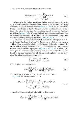
Lf 0 D fðtÞg 5 S FðsÞ 2 S D fð0Þ;
t
t
0
ð11:7Þ
k50
n 2 1 , α # nAN
Unfortunately, the Laplace transform technique used in Riemann Liouville
appears incompatible as it requires the knowledge of the functions fðtÞ having
derivatives at t 5 0of fractional order (Kilbas et al., 1993). But this kind of dif-
ficulty does not occur in the Caputo definition. The Caputo definition for frac-
tional derivative in literature is sometimes named as smooth fractional
derivation (Caputo, 1967). With the help of homogeneous initial conditions
assumption it is established that the systems with Riemann Liouville operators
are similar to those with Caputo operators (Keil et al., 2012).
In literature, for fractional differential equations the appropriate numeri-
cal technique has been developed for those systems which are numerically
stable and can be used for all classes of fractional differential equations. To
use an improved predictor corrector algorithm we choose the Caputo version
for fractional differential equations (Diethelm et al., 2002), in order to get
more precise numerical approximation and reduces computational cost.
Based on the analytical property of the fractional predictor-corrector algo-
rithm the following differential equation:
α
D 5 gðt; xÞ; 0 # t # T
k
k
x ð0Þ 5 x ; k 5 1; 2; :::; m: ð11:8Þ
0
and the voltera integral equation
m21 k ð t
X ðkÞ t 1 gðτ; xÞ
xðtÞ 5 x 0 k! 1 12α dτ ð11:9Þ
k5o ΓðαÞ 0 ðt2τÞ
1
are equivalent. Now set h 5 T=N; t n 5 nhðn 5 0; 1; 2; :::; NAZ Þ
Eq. (11.6) can be rewritten as follows
m21 k α
X ðkÞ t h θ
x h ðt n11 Þ 5 x n11 1 gðt n11 ; x ðt n11 ÞÞ
0 k! h
k50 Γðα 1 2Þ ð11:10Þ
h α X
1 a j;n11 gðt j ; x h ðt j ÞÞ
Γðα 1 2Þ
θ
where x ðt n11 Þ is the predicted value which is determined by
h
n
m21 ðkÞ t k 1 X
θ
X
x ðt n11 Þ 5 x 0 n11 1 b j;n11 gðt j ; x h ðt j ÞÞ
h
k!
k50 ΓðαÞ j50