Page 338 - Mathematical Techniques of Fractional Order Systems

328 Mathematical Techniques of Fractional Order Systems

(A) (B)

40 10

z 1 (t) 20 w 1 (t) 0

0 −10
20 40
20 20
0 0 0 0 20 0 0
20
y (t) −20 −20 x (t) z (t) 0 −20 x 1 (t)
1
1
1
(C) (D)
10 10
w 1 (t) 0 w 1 (t) 0

−10 −10
40 20
20 20
20
20 0 0
0 0 0 0
(t) 0 −20 y (t) Y (t) −20 −20
z 1 1 1 x 1 (t)
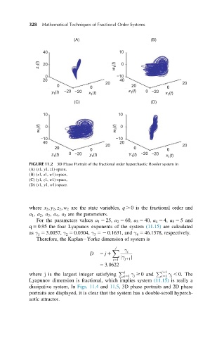
FIGURE 11.2 3D Phase Portrait of the fractional order hyperchaotic Rossler system in
(A) (x1, y1, z1)-space,
(B) (x1, z1, w1)-space,
(C) (y1, z1, w1)-space,
(D) (x1, y1, w1)-space.

where x 2 ; y 2 ; z 2 ; w 2 are the state variables, q . 0 is the fractional order and
a 1 ; a 2 ; a 3 ; a 4 ; a 5 are the parameters.
For the parameters values a 1 5 25; a 2 5 60; a 3 5 40; a 4 5 4; a 5 5 5 and
q 5 0.95 the four Lyapunov exponents of the system (11.15) are calculated
as γ 5 3:0057, γ 5 0:0304, γ 52 0:1631, and γ 5 46:1578, respectively.
1 2 3 4
Therefore, the Kaplan Yorke dimension of system is
j γ
X i
D 5 j 1
jγ
i51 j11 j
5 3:0622
P j P j11
where j is the largest integer satisfying i51 γ $ 0 and i51 γ , 0. The
j
j
Lyapunov dimension is fractional, which implies system (11.15) is really a
dissipative system. In Figs. 11.4 and 11.5, 3D phase portraits and 2D phase
portraits are displayed, it is clear that the system has a double-scroll hyperch-
aotic attractor.