Page 363 - Mathematical Techniques of Fractional Order Systems

354 Mathematical Techniques of Fractional Order Systems

80
60
200
40
150
20
100 0
y 13 (t) 50 y 12 (t) –20
0
–40
–50
100 –60
50 200 –80
0 0 100
–50 –100 –100
(t)
y 12 –100 –200 y (t) –200 –150 –100 –50 0 50 100 150
11
y (t)
11
(A) (B)
160
160
140
140
120
120
100
100
y 13 (t) 80 y 13 (t) 80
60
60
40 40
20 20
0 0
–20 –20
–200 –150 –100 –50 0 50 100 150 –100 –50 0 50 100
y (t) y (t)
11 12
(C) (D)
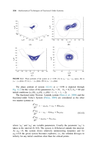
FIGURE 12.2 Phase portraits of Qi system at α 5 0:98: (A) in y 11 2 y 12 2 y 13 space, (B) in
y 11 2 y 12 plane, (C) in y 11 2 y 13 plane, (D) in y 12 2 y 13 plane.
The phase portrait of system (12.11) at α 5 0:98 is depicted through
Fig. 12.2 for the values of the parameters b 11 5 35; b 12 5 8=3; b 13 5 80 and
initial conditions ðy 11 ð0Þ; y 12 ð0Þ; y 13 ð0ÞÞ 5 ð2 1; 2 1; 2 2Þ:
The fractional-order Newton Leipnik system (Sheu et al., 2008) and the
fractional-order Volta’s System (Petras, 2009) are considered as the other
two master systems as
α
d x 21 52 a 21 x 21 1 x 22 1 10x 22 x 23
dt α
α
d x 22
dt α 52 x 21 2 0:4x 22 1 5x 21 x 23 ð12:12Þ
α
d x 23 5 a 22 x 23 2 5x 21 x 22 ;
dt α

where a 21 and a 22 are variable parameters. Usually the parameter a 22 is
0
0
0
0
0
0
taken in the interval (0, 8.0). The system is ill-behaved outside this interval.
As a 22 -0, the system shows relatively uninteresting dynamics and for
a 22 $ 0:8 the given system becomes explosive, i.e., the solution diverges to
infinity for any initial condition other than the critical points.