Page 365 - Mathematical Techniques of Fractional Order Systems

356 Mathematical Techniques of Fractional Order Systems

25
20
10 15
0 10
–10 5
y 23 (t) –20 y 22 (t) 0
–5
–30
–10
–40
40 –15
20 40
–20
0 20
–20 0
y (t) –25
22 –40 –20 (t) –20 –10 0 10 20 30
y 21
y (t)
21
(A) (B)
5 5
0 0
–5 –5
–10 –10
y 23 (t) –15 y 23 (t) –15
–20 –20
–25 –25
–30 –30
–35 –35
–20 –10 0 10 20 30 –30 –20 –10 0 10 20 30
(t) y (t)
y 21 22
(C) (D)
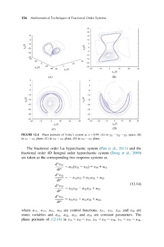
FIGURE 12.4 Phase portraits of Volta’s system at α 5 0:99: (A) in y 21 2 y 22 2 y 23 space, (B)
in y 21 2 y 22 plane, (C) in y 21 2 y 23 plane, (D) in y 22 2 y 23 plane.
The fractional order Lu hyperchaotic system (Pan et al., 2011) and the
fractional order 4D Integral order hyperchaotic system (Deng et al., 2009)
are taken as the corresponding two response systems as
α
d x 31
dt α 5 a 31 ðx 32 2 x 31 Þ 1 x 34 1 u 11
α
d x 32
dt α 52 x 31 x 33 1 a 33 x 32 1 u 12
α ð12:14Þ
d x 33
dt α 5 x 31 x 32 2 a 32 x 33 1 u 13
α
d x 34
5 x 31 x 33 1 a 34 x 34 1 u 14 ;
dt α
where u 11 ; u 12 ; u 13 ; u 14 are control functions, x 31 ; x 32 ; x 33 , and x 34 are
states variables and a 31 ; a 32 ; a 33 , and a 34 are constant parameters. The
phase portraits of (12.14) in x 31 2 x 32 2 x 33 , x 31 2 x 32 2 x 34 , x 31 2 x 33 2 x 34 ,