Page 369 - Mathematical Techniques of Fractional Order Systems

360 Mathematical Techniques of Fractional Order Systems

x 13 ð0ÞÞ 5 ð0:2; 0:5; 0:3Þ, ðy 11 ð0Þ; y 12 ð0Þ; y 13 ð0ÞÞ 5 ð2 1; 2 1; 2 2Þ, ðx 21 ð0Þ;
x 22 ð0Þ; x 23 ð0ÞÞ 5 ð0:19; 0; 2 0:18Þ, ðy 21 ð0Þ; y 22 ð0Þ; y 23 ð0ÞÞ 5 ð8; 2; 3Þ and
slave systems Lu hyperchaotic system, 4D Integral order hyperchaotic system
are taken as ðx 31 ð0Þ; x 32 ð0Þ; x 33 ð0Þ; x 34 ð0ÞÞ 5 ð2 10; 2 14; 12; 10Þ and
ðy 31 ð0Þ; y 32 ð0Þ; y 33 ð0Þ; y 34 ð0ÞÞ 5 ð1:2; 0:6; 0:8; 0:5Þ, respectively. Hence
the initial condition of the error system will be ðe 11 ð0Þ; e 12 ð0Þ;
e 13 ð0Þ; e 14 ð0Þ; e 21 ð0Þ; e 22 ð0Þ; e 23 ð0Þ; e 24 ð0ÞÞ 5 ð2 10:39; 2 14:50; 11:88;
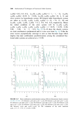
9:88; 2 5:80; 2 4; 2 2; 2 0:5Þ. Fig. 12.7A H show the chaotic systems
are dual combination synchronized and it is also seen from Fig. 12.7I that the
error vectors asymptotically converge to zero as time becomes large which
implies that dual combination synchronizations among the considered frac-
tional order systems are achieved at α 5 0:98.

30 40
x (t) x (t)
31 32
x (t)+x (t) x (t)+x (t)
21 11 30 22 21
20
20
10
x 31 (t), x 21 (t)+x 11 (t) 0 x 32 (t), x 22 (t)+x 12 (t) 10 0
–10
–10
–20
–20
–30 –30
0 1 2 3 4 5 6 7 8 9 10 0 1 2 3 4 5 6 7 8 9 10
t t
(A) (B)
60 60
x (t) x (t)
33 34
x (t)+x (t) x (t)+x (t)
23 13 23 13
50 50
40
40
x 33 (t), x 23 (t)+x 13 (t) 30 x 34 (t), x 23 (t)+x 13 (t) 30
20
20
10 10
0 0
0 1 2 3 4 5 6 7 8 9 10 0 1 2 3 4 5 6 7 8 9 10
t t
(C) (D)
FIGURE 12.7 Dual combination synchronization among different dimensional chaotic systems
(12.10) (12.15) : (A) between x 31 ðtÞ and x 21 ðtÞ 1 x 11 ðtÞ; (B) between x 32 ðtÞ and x 22 ðtÞ 1 x 12 ðtÞ;
(C) between x 33 ðtÞ and x 23 ðtÞ 1 x 13 ðtÞ; (D) between x 34 ðtÞ and x 23 ðtÞ 1 x 13 ðtÞ; (E) between y 31 ðtÞ
and y 21 ðtÞ 1 y 11 ðtÞ; (F) between y 32 ðtÞ and y 22 ðtÞ 1 y 12 ðtÞ; (G) between y 33 ðtÞ and y 23 ðtÞ 1 y 13 ðtÞ;
(H) between y 34 ðtÞ and y 23 ðtÞ 1 y 13 ðtÞ; (I) The evaluation of the error functions
e ji ðtÞ; j 5 1; 2; i 5 1; 2; 3; 4at α 5 0:98.