Page 436 - Mathematical Techniques of Fractional Order Systems

Applications of Continuous-time Fractional Order Chapter | 14 421

and nonlinear control. The master and slave configuration for both schemes
can be written as:
α
α
α
3
D x 1 52 vðx 2 μx 1 2 y 1 Þ; D y 1 5 x 1 2 γy 1 2 z 1 ; D z 1 5 βy 1 ; ð14:33Þ
1
and:
α 3 α α
D x 2 52 vðx 2 μx 2 2 y 2 Þ 2 u 1 ; D y 2 5 x 2 2 γy 2 2 z 2 2 u 2 ; D z 2 5 βy 2 2 u 3 :
2
ð14:34Þ
In the case of linear feedback error coupling, the control signals are
defined as:
u 1 5 k 1 ðx 2 2 x 1 Þ; u 2 5 k 2 ðy 2 2 y 1 Þ; u 3 5 k 3 ðz 2 2 z 1 Þ: ð14:35Þ

The synchronization gains were chosen so as to satisfy the conditions
given in (Jiang et al., 2003): k 1 5 280, k 2 5 250, and k 3 5 100. For the other
synchronization scheme (nonlinear control), the controllers were:

Þðx 1 2 x 2 Þ; u 2 5 u 2 3 5 0;
u 1 5 ðk 1 1 μk x 1 ;x 2 ð14:36Þ
2
2
5 x 1 x 1 x 2 1 x $ 0. The error dynamics of the systems is
1 2
where k x 1 ;x 2
reduced to (Matouk, 2011):
α
α
α
D e x 52 vð2 μe x 2 e y Þ 1 k 1 e x ; D e y 5 e x 2 γe y 2 e z ; D e z 5 βe y : ð14:37Þ
The gain k 1 5 69:211 was chosen such that the fractional order error sys-
tem is locally asymptotically stable and tends to the zero equilibrium point.
This means that the master and slave systems can synchronize.
14.4.2 Synchronization of Electrically Coupled Neuron Systems
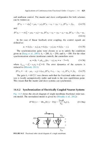
Fig. 14.5 shows the circuit diagram of single membrane fractional order neu-
ron model. The normalized model is given by (Moaddy et al., 2012):
α
D XðτÞ 52 Rσ m XðτÞ 2 YðtÞ 1 2πaR I m ðτÞ; ð14:38aÞ
V R

FIGURE 14.5 Fractional order circuit diagram of a single membrane.