Page 479 - Mathematical Techniques of Fractional Order Systems

Multiswitching Synchronization Chapter | 15 465

3
–0.05
2 –0.1
y 1 ,x 1 1 y 1 - x 1 –0.15

0 –0.2
–1 –0.25
20 40 60 80 100 0.5 1 1.5 2
t t ×10 4

2
–0.2
y 1 ,x 2 0 y 1 - x 2 –0.4
–0.6
–2
–0.8
–4 –1
20 40 60 80 100 0.5 1 1.5 2
t t ×10 4

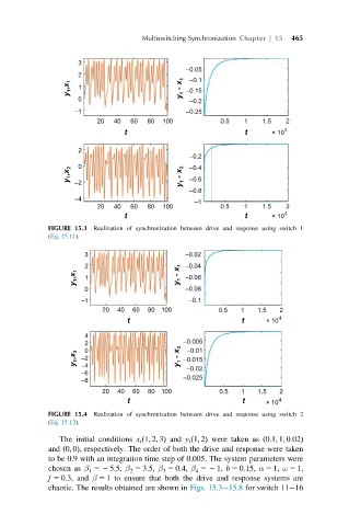
FIGURE 15.3 Realization of synchronization between drive and response using switch 1
(Eq. 15.11).

3 –0.02
2 –0.04
y 1 ,x 1 1 y 1 - x 1 –0.06
0 –0.08
–1 –0.1
20 40 60 80 100 0.5 1 1.5 2
t t ×10 4
4
2 0 –0.005
–0.01
y 1 ,x 3 –2 y 1 - x 3 –0.015
–4
–6 –0.02
–8 –0.025
20 40 60 80 100 0.5 1 1.5 2
t t ×10 4
FIGURE 15.4 Realization of synchronization between drive and response using switch 2
(Eq. 15.12).

The initial conditions x i ð1; 2; 3Þ and y i ð1; 2Þ were taken as ð0:1; 1; 0:02Þ
and ð0; 0Þ, respectively. The order of both the drive and response were taken
to be 0.9 with an integration time step of 0:005. The system parameters were
chosen as β 52 5:5, β 5 3:5, β 5 0:4, β 52 1, b 5 0:15, α 5 1, ω 5 1,
4
2
1
3
f 5 0:3, and β 5 1 to ensure that both the drive and response systems are
chaotic. The results obtained are shown in Figs. 15.3 15.8 for switch 11 16