
Page 640 - Mathematical Techniques of Fractional Order Systems
P. 640
Enhanced Fractional Order Chapter | 20 611
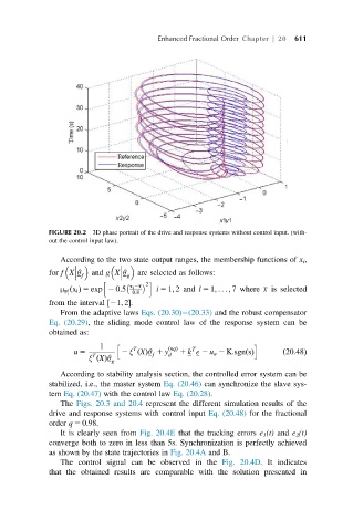
FIGURE 20.2 3D phase portrait of the drive and response systems without control input. (with-
out the control input law).
According to the two state output ranges, the membership functions of x i ,
are selected as follows:
for fX θ f and gX θ g
h 2 i
x i 2x
μ l x i 5 exp 2 0:5 0:8 i 5 1; 2 and l 5 1; ... ; 7 where x is selected
ðÞ
F
i
from the interval 21; 2.
½
From the adaptive laws Eqs. (20.30) (20.33) and the robust compensator
Eq. (20.29), the sliding mode control law of the response system can be
obtained as:
1 h T T i
u 5 2 ξ XðÞθ 1 y ð d nqÞ 1 k e 2 u a 2 K:sgnðsÞ ð20:48Þ
f
ξ ðXÞθ
T
g
According to stability analysis section, the controlled error system can be
stabilized, i.e., the master system Eq. (20.46) can synchronize the slave sys-
tem Eq. (20.47) with the control law Eq. (20.28).
The Figs. 20.3 and 20.4 represent the different simulation results of the
drive and response systems with control input Eq. (20.48) for the fractional
order q 5 0.98.
It is clearly seen from Fig. 20.4E that the tracking errors e 1 (t) and e 2 (t)
converge both to zero in less than 5s. Synchronization is perfectly achieved
as shown by the state trajectories in Fig. 20.4A and B.
The control signal can be observed in the Fig. 20.4D. It indicates
that the obtained results are comparable with the solution presented in