Page 637 - Mathematical Techniques of Fractional Order Systems

608 Mathematical Techniques of Fractional Order Systems

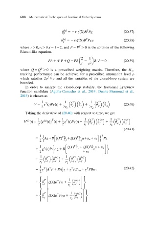
θ ðqÞ 52 r 1 ξðXÞB Pe
T
f ð20:37Þ
T
θ ðqÞ 52 r 2 ξðXÞB Peu
g ð20:38Þ
T
where r . 0; r i . 0; i 5 1B2, and P 5 P . 0 is the solution of the following
Riccati-like equation.

2 1 T
T
PA 1 A P 1 Q 2 PB 2 B P 5 0 ð20:39Þ
r ρ 2
T
where Q 5 Q . 0 is a prescribed weighting matrix. Therefore, the H N
tracking performance can be achieved for a prescribed attenuation level ρ
2
which satisfies 2ρ $ r and all the variables of the closed-loop system are
bounded.
In order to analyze the closed-loop stability, the fractional Lyapunov
function candidate (Aguila-Camacho et al., 2014; Duarte-Mermoud et al.,
2015) is chosen as
1 1 T 1 T
T
V 5 e tðÞPetðÞ 1 θ ~ f θ ~ f 1 θ ~ g ~ θ g ð20:40Þ
2 2r 1 2r 2
Taking the derivative of (20.40) with respect to time, we get
T 1 T 1 ~ T ~ ðqÞ 1 ~ T ~ ðqÞ
1
V ðÞ 5 e ðÞ ðÞ 1 e tðÞPetðÞ 1 θ f θ f 1 θ g θ g
t
q ðÞ
t
q ðÞ
t
2 2 r 1 r 2
ð20:41Þ
1 n h T ~ T ~ io T
5 Ae1B ξ XðÞ θ 1ξ XðÞ θ u1u a 1w 1 Pe
2 f g
1 T ~ T ~
T
1 e eðÞPAe 1 B ξ XðÞ θ 1 ξ XðÞ θ u 1 u a
f
g
2 1w 1
1 T q ðÞ 1 T q ðÞ
1 θ ~ θ ~ 1 θ ~ θ ~
r 1 f f r 2 g g
1
T
T
T
T
5 e A P 1 PA e 1 e PBu a 1 e PBw 1 ð20:42Þ
2
8 39
2
< T 1 =
T
1 θ ~ 4 ξ XðÞB Pe 1 θ ~ ðqÞ 5
f f
r 1
: ;
8 2 39
< T 1 ðqÞ =
ðÞB Peu 1
1 θ ~ 4 ξ X T θ ~ 5
g g
: r 2 ;