Page 681 - Mathematical Techniques of Fractional Order Systems

652 Mathematical Techniques of Fractional Order Systems

parameters (a 5 0.5, b 5 0.2, c 5 10) and orders p 1 5 p 2 5 p 3 5 p,using the
relation (21.15), we can verify that for 0.9 # p # 1 the system is chaotic
with a positive Lyapunov exponent 0.0368. The minimal commensurate
order from which the system (21.21) can exhibit a chaotic behavior is
p . 0.839.
For first example, if it is assumed that the commensurate order has an
arbitrary fixed values p 1 5 p 2 5 p 3 5 p 5 0.95, parameters are chosen as
(a 5 0.5, b 5 0.2, c 5 10), initial conditions are selected as (x 0 520.5,
y 0 5 0, z 0 5 1), and computational time 100s for time step h 5 0.01, then the
fractional order Ro ¨ssler’s system (21.21) satisfies the condition of presence
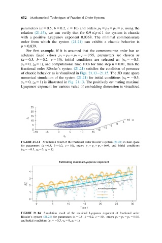
of chaotic behavior as is visualized in Figs. 21.13 21.15. The 3D state space
numerical simulation of the system (21.21) for initial conditions (x 0 520.5,
y 0 5 0, z 0 5 1) is illustrated in Fig. 21.13. The positively estimating maximal
Lyapunov exponent for various value of embedding dimension is visualized

25
20
15
z t
10 10 y t
5
0
5 –5
–10
0 –15
–10 –5 0 5 10 15
x t
FIGURE 21.13 Simulation result of the fractional order Ro ¨ssler’s system (21.21) in state space
for parameters (a 5 0.5, b 5 0.2, c 5 10), orders p 1 5 p 2 5 p 3 5 0.95, and initial conditions
(x 0 520.5, y 0 5 0, z 0 5 1).

Estimating maximal Lyapunov exponent

4
3
S(t) 2

Embedding dimension
1 5
6
0 7
0 5 10 15 20 25 30
Time t
FIGURE 21.14 Simulation result of the maximal Lyapunov exponent of fractional order
Ro ¨ssler’s system (21.21) for parameters (a 5 0.5, b 5 0.2, c 5 10), orders p 1 5 p 2 5 p 3 5 0.95,
and initial conditions (x 0 520.5, y 0 5 0, z 0 5 1).