Page 676 - Mathematical Techniques of Fractional Order Systems

Fractional Order Chaotic Systems Chapter | 21 647

20406080 100

z t 20 40 60 y t

–40 –20 0
0 –60
–40 –30 –20 –10 0 10 20 30 40
x t
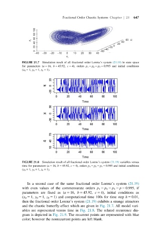
FIGURE 21.7 Simulation result of all fractional order Lorenz’s system (21.19) in state space
for parameters (a 5 16, b 5 45.92, c 5 4), orders p 1 5 p 2 5 p 3 5 0.995 and initial conditions
(x 0 5 1, y 0 5 1, z 0 5 1).

FIGURE 21.8 Simulation result of all fractional order Lorenz’s system (21.19) variables versus
time for parameters (a 5 16, b 5 45.92, c 5 4), orders p 1 5 p 2 5 p 3 5 0.995 and initial conditions
(x 0 5 1, y 0 5 1, z 0 5 1).

In a second case of the same fractional order Lorenz’s system (21.19)
with even values of the commensurate orders p 1 5 p 2 5 p 3 5 p 5 0.995, if
parameters are fixed as (a 5 16, b 5 45.92, c 5 4), initial conditions as
(x 0 5 1, y 0 5 1, z 0 5 1) and computational time 100s for time step h 5 0.01,
then the fractional order Lorenz’s system (21.19) exhibits a strange attractors
and the chaotic butterfly-effect which are given in Fig. 21.7. All model vari-
ables are represented versus time in Fig. 21.8. The related recurrence dia-
gram is depicted in Fig. 21.9. The recurrent points are represented with blue
color; however the nonrecurrent points are left blank.