Page 228 - Matrix Analysis & Applied Linear Algebra

4.6 Classical Least Squares 223
4.6 CLASSICAL LEAST SQUARES

The following problem arises in almost all areas where mathematics is applied.
At discrete points t i (often points in time), observations b i of some phenomenon
are made, and the results are recorded as a set of ordered pairs
D = {(t 1 ,b 1 ), (t 2 ,b 2 ),. . . , (t m ,b m )} .
On the basis of these observations, the problem is to make estimations or predic-
tions at points (times) ˆ t that are between or beyond the observation points t i .
A standard approach is to find the equation of a curve y = f(t) that closely fits
the points in D so that the phenomenon can be estimated at any nonobservation
y
point ˆ t with the value ˆ = f( ˆ t).
Let’s begin by fitting a straight line to the points in D. Once this is under-
stood, it will be relatively easy to see how to fit the data with curved lines.
(t m ,b m )
b •

ε m
f (t)= α + βt
• •

t m ,f (t m )
•
(t 2 ,b 2 )
•
•
• t
•
ε 2
•
t 1 ,f (t 1 )

• t 2 ,f (t 2 ) •
ε 1

•
(t 1 ,b 1 )
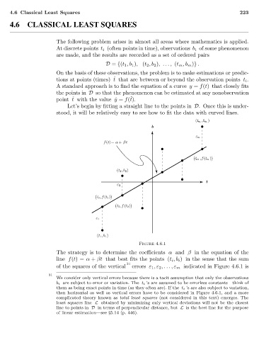
Figure 4.6.1
The strategy is to determine the coefficients α and β in the equation of the
line f(t)= α + βt that best fits the points (t i ,b i ) in the sense that the sum
31
of the squares of the vertical errors ε 1 ,ε 2 ,...,ε m indicated in Figure 4.6.1 is
31
We consider only vertical errors because there is a tacit assumption that only the observations
b i are subject to error or variation. The t i ’s are assumed to be errorless constants—think of
them as being exact points in time (as they often are). If the t i ’s are also subject to variation,
then horizontal as well as vertical errors have to be considered in Figure 4.6.1, and a more
complicated theory known as total least squares (not considered in this text) emerges. The
least squares line L obtained by minimizing only vertical deviations will not be the closest
line to points in D in terms of perpendicular distance, but L is the best line for the purpose
of linear estimation—see §5.14 (p. 446).