Page 27 - Mechanical Engineers Reference Book

1/16 Mechanical engineering principles
where P(x + Ax) - P(x) is the probability that the value of
x(t) will lie between x and x + Ax (Figure 1.27). Now
dP(4
P(4 =
so that

P(4 = I_:P(xW
Hence
I:
P(w) = p(x)dx = 1
so that the area under the probability density function curve is
unity.
A random process is stationary if the joint probability
density
P(X(tl), x(t2), x(t3), ’ ’ ’ 1
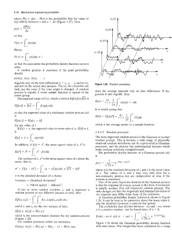
depends only on the time differences t2 - tl, t3 - t2 and so on, Figure 1.28 Random processes
and not on the actual time instants. That is, the ensemble will
look just the same if the time origin is changed. A random
process is ergodic if every sample function is typical of the since the average depends only on time differences. If the
entire group. process is also ergodic, then
The expected value off(x), which is written E&)] orf(x) is

It is worth noting that
so that the expected value of a stationary random process x(t)
is
E[X(tl)l = Wtl + 41
for any value of t. which is the average power in a sample function
Iff@) = x, the expected value or mean value of x, E[x] or X,
is 1.4.3.3 Random processes
re
~[x] = J-, xp(x)d~ The most important random process is the Gaussian or normal
=
random process. This is because a wide range of physically
r : make analysis relatively straightforward.
In addition, if f(x) = x2, the mean square value of x, j2 is observed random waveforms can be represented as Gaussian
processes, and the process has mathematical features which
E[x2] = 2 = xz . p(x)dx The probability density function of a Gaussian process x(t)
The variance of x, cr2 is the mean square value of x about the is
mean, that is,
r-
cr2 = E[(x - 421 = 1 (x - X)2p(x)dx = (x2) - ($2 where u is the standard deviation of x and X is the mean value
J-, of x. The values of u and X may vary with time for a
cr is the standard deviation of x, hence non-stationary process but are independent of time if the
Variance = (Standard deviation)2 process is stationary.
One of the most important features of the Gaussian process
= {Mean square - (Mean)’} is that the response of a linear system to this form of excitation
is usually another (but still Gaussian) random process. The
If two or more random variables XI and x2 represent a only changes are that the magnitude and standard deviation of
random process at two different instants of time, then
the response may differ from those of the excitation.
A Gaussian probability density function is shown in Figure
Elf(XlrX2)I = j-: j-: f(XliX21P(~l>XZ)~l~2 1.29. It can be seen to be symmetric about the mean value 1,
and the standard deviation u controls the spread.
and if tl and t2 are the two instants of time, The probability that x(t) lies between -Am and +Au, where
A is a positive number, can be found since, if X = 0,
E[x(t1), x(t2)l = R(tl>t’)
which is the autocorrelation function for the random process
(Figure 1.28).
For random processes which are stationary, Figure 1.30 shows the Gaussian probability density function
E[x(td, ~(t2)l = R(td2) = R(t2 - tl) = R(.i), say, with zero mean. This integral has been calculated for a range