Page 28 - Mechanical Engineers Reference Book

Vibrations 1/17

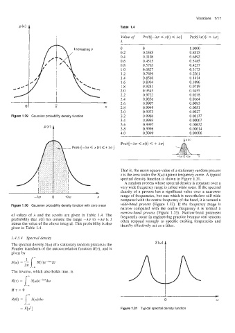
Table 1.4
Value of Prob[-Aa C x(t) < hu] Prob[lx(t)/ > Ag]
A
~
0 0 1.0000
0.2 0.1585 0.8415
0.4 0.3108 0.6892
0.6 0.4515 0.5485
0.8 0.5763 0.4237
1.0 0.6827 0.3173
1.2 0.7699 0.2301
1.4 0.8586 0.1414
1.6 0.8904 0.1096
1.8 0.9281 0.0719
2.0 0.9545 0.0455
2.2 0.9722 0.0278
- 2.4 0.9836 0.0164
2.6
0.9907
0.0093
X 2.8 0.9949 0.0051
3.0 0.9973 0.0027
Figure 11.29 Gaussian probability density function 3.2 0.9986 0.00137
3.4 0.9993 0.00067
3.6 0.9997 0.00032
3.8 0.9998 0.00014
4.0 0.9999 0.00006
Prob[-Ar x(t) < + Ar]
Pro$ {-Xu < x(t) <+ha}
-XoO+ho X

That is, the mean square value of a stationary random process
x is the area under the S(w) against frequency curve. A typical
spectral density function is shown in Figure 1.31.
A random process whose spectral density is constant over a
very wide frequency range is called white noise. If the spectral
density of a process has a significant value over a narrower
-XU 0 +XU X range of frequencies, but one which is nevertheless still wide
compared with the centre frequency of the band, it is termed a
Figure 1.30 Gaussian probability density function with zero mean wide-band process (Figure 1.32). If the frequency range is
narrow compared with the centre frequency it is termed a
narrow-band process (Figure 1.33). Narrow-band processes
of values of A and the results are given in Table 1.4. The frequently occur in engineering practice because real systems
probability that x(t) lies outside the range --hr to +ACT is 1 often respond strongly to specific exciting frequencies and
minus the value of the above integral. This probability is also thereby effectively act as a filter.
given in Table 1.4.

1.4.3.4 Spectral density
The spectral decsity S(w) of a stationary random process is the
Fourier. transform of the autocorrelation function R(T), and is
given by
1 -
S(w) = ~1- R(~)e-'~'d7
The inverse, which also holds true, is
1:
R(T) = S(w)e-'wrd~
If.r=O
i:
R(0) = S(w)dw 0
= E[x2] Figure 1.31 Typical spectral density function