Page 34 - Mechanical Engineers Reference Book

Mechanics of fluids 1/23
2: is the height above some datum, Integration for a constant-density fluid gives:
v is the mean velocity of flow.
Vi
Specific means ‘per unit mass’. For non-steady flow condi- + - + gz = constant (1.36)
tions, either quasi-steady techniques or the integration of P 2
infinitely small changes may be employed.
These energy per unit mass terms may be converted to energy
per unit weight terms, or heads, by dividing by g to give:
(h) Momentum Momentum is the product of mass and
velocity (mv). Newton’s laws of motion state that the force P VL
applied to a system may be equated to the rate of change of - + - + Z = constant (1.37)
%
momentum of the system, in the direction of the force. The Pg
change in momentum may be related to time andor displace- which is the Bernoulli (or constant head) equation.
ment. In a steady flow situation the change related to time is These equations are the generally more useful simplifica-
zero, so the change of momentum is usually taken to be the tions of the Navier-Stokes equation:
product of the mass flow rate and the change in velocity with Dv
displacement. Hence the force applied across a system is _- pB - op + V{U(VV + VE)} (1.38)
-
Dt
F = mAv (1.30)
where B is the body force and E the rate of expansion
where Av is the change in velocity in the direction of the force
F.
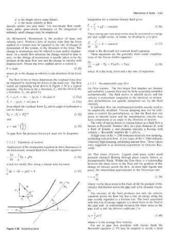
For flow in two or three dimensions the resultant force may
be obtained by resolving the forces in the usual way. The flow 1.5.3.3 Incompressible pipe flow
round an expanding bend shown in Figure 1.39 is a typical
example. The force in the x direction, Fx, and the force in the (a) Flow regimes The two major flow regimes are laminar
y direction, Fy, are given by and turbulent. Laminar flow may be fairly accurately modelled
mathematically. The fluid moves in smooth layers and the
F, = plAi + Av, - (pzAz + &V,)COS 0 (1.31a) velocity is everywhere tangential to the direction of motion.
Any perturbations are quickly dampened out by the fluid
Fy = -(pzAz + &&in 0 (1.31b) viscosity.
from which the resultant force FR and its angle of inclination a In turbulent flow the mathematical models usually need to
can be f’ound: be empirically modified. Viscous damping may not be suffi-
FR = {F: + F;}’.’ (1.32) cient to control the perturbations, so that the fluid does not
move in smooth layers and the instantaneous velocity may
and have components at an angle to the direction of motion.
The ratio of inertia forces to viscous forces in a fluid flow is
(1.33) known as Reynolds’ Number (Re). In a pipe diameter D, with
a fluid of density p and dynamic viscosity 7) flowing with
In pipe flow the pressure forces pR must not be forgotten. velocity v, Reynolds’ number Re = pDvlv.
A high value of Re > 2300 indicates relatively low damping,
predicting turbulent flow. A low value of Re < 2GOO indicates
1.5.3.2 Equations of motion relatively high damping, predicting laminar flow. These values
were suggested in an historical experiment by Osborne Rey-
Application of the momentum equation in three dimensions to nolds.
an irrotational, inviscid fluid flow leads to the Euler equation:
1 (6) Pipe losses (friction) Liquids (and gases under small
- !? = - ‘Vp + gOh (1.34) pressure changes) flowing through pipes usually behave as
Dt P incompressible fluids. Within the flow there is a relationship
which for steady flow along a stream tube becomes: between the shear stress in the fluid and the gradient of the
change of velocity across the flow. In most light liquids and
1 gases, the relationship approximates to the Newtonian one:
- dp + lvdv + gdZ = 0 (1.35)
P
(1.39)

where Tis the shear stress in the fluid, dvldy the gradient of the
velocity distribution across the pipe and 9 the dynamic viscos-
ity.
The viscosity of the fluid produces not only the velocity
variation across the flow but also a loss of energy along the
pipe usually regarded as a friction loss. The force associated
with this loss of energy appears as a shear force in the fluid at
the pipe wall. A relationship between the shear stress at the
pipe wall T,, and the friction coefficient, f is:
1
/ ro = - pv2f (1.40)
2
/’ where v is the average flow velocity.
For use in pipe flow problems with viscous fluids the
Figure 1.39 Expanding bend Bernoulli equation (1.37) may be adapted to incude a head