Page 56 - Mechanical Engineers Reference Book

Heat transfer 1145
.
In free (convection the relationship used is Nu = ~(PY Gr)
where Gv is the Grashof number, p2pgO13/p2 in which p is the
coefficient of cubical expansion of the fluid and O is a
temperature difference (usually surface to free stream tempe-
rature). The transition from laminar to turbulent flow is
determiined by the product (Pr . Gr) known as the Rayleigh
number, Ra. As a simple example, for plane or cylindrical,
vertical surfaces it is found that;
For Ra < IO9, flow is laminar and Nu = O.59(Pr . Gr)0.25
For Ra > lo9, flow is turbulent and Nu = 0.13(Pr. Gr)1’3
The 1-epresentative length dimension is height and the
resulting heat transfer coefficients are average values for the
whole height. Film temperature is used for fluid properties.
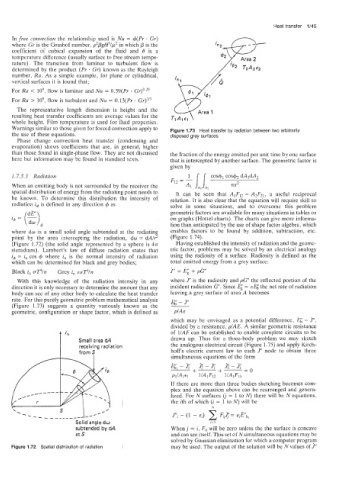
Warnings similar to those given for forced convection apply to Figure 1.73 Heat transfer by radiation betweer: two arbitrarily
the use of these equations. disposed grey surfaces
Phase change convection heat transfer (condensing and
evaporation) shows coefficients that are, in general, higher
than those found in single-phase flow. They are not discussed the fraction of the energy emitted per unit time by one surface
here bul. information may be found in standard texts. that is intercepted by another surface. The geometric factor is
given by
1.7.3.3 Radiation Fl2 = J AI j-
cos+, cos+, dAldA2
When an emitting body is not surrounded by the receiver the A? TX2
spatial distribution of energy from the radiating point needs to It can be seen that AIFlz = A*F2,, a useful reciprocal
be known. To determine this distribution the intensity of relation. It is also clear that the equation will require skill to
radiation id is defined in any direction 4 as solve in some situations, and to overcome this problem
geometric factors are available for many situations in tables or
on graphs (Hottel charts). The charts can give more informa-
tion than anticipated by the use of shape factor algebra, which
where dw is a small solid angle subtended at the radiatin enables factors to be found by addition, subtraction, etc.
point by the area i2tercepting the radiation, dw = dA/ $ (Figure 1.74).
(Figure 1.72) (the solid angle represented by a sphere is 47r Having established the intensity of radiation and the geome-
steradiains). Lambert’s iaw of diffuse radiation states that tric factor, problems may be solved by an electrical analogy
i, = in cos 4 where in is the normal intensity of radiation using the radiosity of a surface. Radiosity is defined as the
which can be determined for black and grey bodies; total emitted energy from a grey surface:
Black in rp/.ir Grey in mpln J = p; + p&
With this knowledge of the radiation intensity in any where .?’ is the radiosity and,p& the reflected portion of the
direction it is only necessary to determine the amount that any incident radiation G. Since E: = &E{ the net rate of radiation
body cain see of any other body to calculate the heat transfer leaving a grey surface of area A becomes
rate. For this purely geometric problem mathematical analysis
(Figure 1.73) suggests a quantity variously known as the
geometric, configuration or shape €actor, which is defined as p/A E
which may be envisaged as a potential difference, &[ - 2,
divided by a resistance, p/AE. A similar geometric resistance
of 1IAF can be established to enable complete circuits to be
Small area ciA drawn up. Thus for a three-body problem we may sketch
receiving radiation the analogous electrical circuit (Figure 1.75) and apply Kirch-
from S hoff‘s electric current law to each s’ node to obtain three
simultaneous equations of the form
E{,-$ 3-4 p 3- p 1
+-+-- -0
P1IA1EI 1IA1F12 1IA1F13
If there are more than three bodies sketching becomes com-
plex and the equation above can be rearranged and genera-
lized. For N surfaces (j = 1 to N) there will be N equations,
the ith of which (i = 1 to N) will be
“j
Yi - (1 - E!) Fij$ = qEb,
,=1
subtended by d.4 When j = i, Fli will be zero unless the the surface is concave
at S and can see itself. This set of N simultaneous equations may be
solved by Gaussian elimination for which a computer program
Figure 1.72 Spatial distribution of radiation may be used. The output of the solution will be N values of S‘