Page 55 - Mechanical Engineers Reference Book

1/44 Mechanical engineering principles
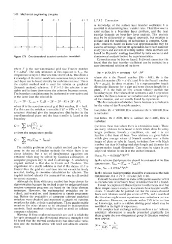
1 2 3 n-I n n+l 1.7.3.2 Convection
A knowledge of the surface heat transfer coefficient h is
essential in determining heat transfer rates. Fluid flow over a
solid surface is a boundary layer problem, and the heat
transfer depends on boundary layer analysis. This analysis
may be by differential or integral approach, but solution is
difficult and the modelling of turbulence is complex. Com-
puter solutions based on numerical approximations may be
used to advantage, but simple approaches have been used for
many years and are still extremely useful. These methods are
based on Reynolds' analogy (modified by later workers) and
Figure 1.71 One-dimensional transient conduction formulation dimensional analysis backed by experimentation.
Convection may be free or forced. In forced convection it is
found that the heat transfer coefficient can be included in a
non-dimensional relation of the form
where F is the non-dimensional grid size Fourier number
F = aAt/a2. The only unknown in this equation is Tn,l, the Nu = +(Re,Pr) = constant . Re" . Prb
temperature at layer n after one time internval At. Thus from a
knowledge of the initial conditions successive temperatures in where Nu is the Nusselt number (Nu = hNk), Re is the
each layer can be found directly for each time interval. This is Reynolds number (Re = pvZ/~) and Pr is the Prandtl number
the explicit method and is used for tabular or graphical (Pr = pcp/k). In these relations 1 is a representative length
(Schmidt method) solutions. If F > 0.5 the solution is un- dimension (diameter for a pipe and some chosen length for a
stable and in three dimensions the criterion becomes severe. plate), V is the bulk or free stream velocity outside the
The boundary conditions may be isothermal or convective and boundary layer. The values of the constants a and b depend on
in the latter case the solution is whether the flow is laminar or turbulent and on the geometry
of the situation, and are usually found by experiment.
The determination of whether flow is laminar or turbulent is
where B is the non-dimensional grid Biot number, B = ha/k. by the value of the Reynolds number;
For this case the solution is unstable if (F + FB) > 0.5. The For plates', Re < 500 000, flow is laminar: Re > 500 000, flow
solutions obtained give the temperature distribution in the is turbulent
one-dimensional plane and the heat transfer is found at the
boundary For tubes, Re < 2000, flow is laminar: Re > 4000, flow is
turbulent
(between these two values there is a transition zone). There
are many relations to be found in texts which allow for entry
or from the temperature profile length problems, boundary conditions, etc. and it is not
feasible to list them all here. Two relations are given below
which give average values of Nusselt number over a finite
Q = mCp(Tfina1 - Tinitial) length of plate or tube in forced, turbulent flow with Mach
layer
number less than 0.3 using total plate length and diameter for
The stability problems of the explicit method can be over- representative length dimension. Care must be taken in any
come by the use of implicit methods for which there is no empirical relation to use it as the author intended.
direct solution, but a set of simultaneous equations are
obtained which may be solved by Gaussian elimination. A Plate; Nu = 0.036Re0.*Pr0 33
computer program may be used to advantage. A satisfactory In this relation fluid properties should be evaluated at the film
implicit method is that due to Crank and Nicolson. The temperature, Tfilm = (TWaLl + Tbulk)/2.
importance of a stable solution is that if the choice of F is
limited then the grid size and time interval cannot be freely Tube; Nu = 0.023Re0.8Pr0.4
selected, leading to excessive calculations for solution. The In this relation fluid properties should be evaluated at the bulk
implicit method releases this constraint but care is still needed temperature, 0.6 < Pr < 160 and (l/d) > 60.
to ensure accuracy. It should be noted that the index of Reynolds number of 0.8
Although the finite difference method has been chosen for is characteristic of turbulent flow; in laminar flow 0.5 is found.
demonstration because the method is easy to understand most It must be emphasized that reference to other texts in all but
modern computer programs are based on the finite element these simple cases is essential to estimate heat transfer coeffi-
technique. However, the mathematical principles are in- cients. It should also be pointed out that the values obtained
volved, and would not lend themselves to simple programm- from such relations could give errors of 25%, and a search of
ing. Before the availability of computer software analytical the literature might reveal equations more suited to a particu-
solutions were obtained and presented as graphs of transient lar situation. However, an estimate within 25% is better than
solutions for slabs, cylinders and spheres. These graphs enable no knowledge, and is a suitable starting point which may be
solutions for other shapes to be obtained by superposition modified in the light of experience.
methods. Such methods should be used to avoid or validate For complex heat exchange surfaces such as a car radiator,
computer solutions. empirical information is usually presented graphically (on
Warning: If fibre-reinforced materials are used in which the these graphs the non-dimensional group St (Stanton number)
lay-up is arranged to give directional structural strength it will may appear:
be found that the thermal conductivity has directional varia-
Nu
tion and the methods above will need considerable amend- St=--- - h
ment. RePr pVcp