Page 54 - Mechanical Engineers Reference Book

Heat transfer 1/43
1-73 Analysis of heat transfer1&16
1.7.3.1 Conduction Y
By considering the thermal equilibrium of a small, three-
dimensional element of solid, isotropic material it can be a
shown that for a rectangular coordinate system

where aT/& is the rate of change of temperature with tjme, 01 is
the thermal diffusivity of the material LY = k/pcp and Q”‘ is the w
internal heat generation rate per unit volume, which may be
due, for example, to electric current flow for which Q”’ = i2r,
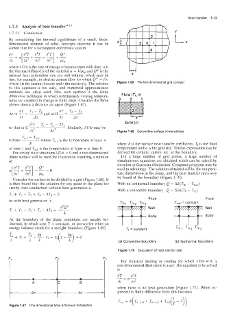
where i is the current density and r the resistivity. The solution Figure 1.68 The two-dimensional grid concept
to this equation is Cot easy, and numerical approximation
methods are often used. One such method is the finite
difference technique in whicn continuously varying tempera-
tures are assumed to change in finite steps. Consider the three
planes shown a distance Ax apart (Figure 1.67).
aT T~ - T~ dT 72 - T;
=
At A -- = ~ and at B - -
ax Ax ax AX
dZT TI + T; - 2T2 Solid (k)
so that at C- = . Similarly. aTldt may be
ax2 AX2 Figure 1.69 Convective surface nomenclature
written TnJ - Trl.0 where T, is the temperature at layer n
dt where h is the surface heat transfer coefficient, Tf is the fluid
at time 1 and Tfl,o is the temperature at layer n at time 0. temperature and a is the grid size. Similar expressions can be
For steady state situations 8Tldt = 0 and a two-dimensional derived for corners, curves, etc. at the boundary.
plane surface will be used for illustration requiring a solution For a large number of grid points, a large number of
of simultaneous equations are obtained which can be solved by
iteration or Gaussian elimination. Computer programs may be
used to advantage. The solution obtained will be the tempera-
ture distribution in the plane, and the heat transfer rates may
be found at the boundary (Figure 1.70):
Consider the surface to be divided by a grid (Figure 1.68). It
is then found that the solution for any point in the plane for With an isothermal boundary Q = Hk(T, - TWalJ
steady state conduction without heat generation is
With a convective boundary 0 = Bha(Tf - T,)
Ti + T; + T3 + Td - 4To = 0
or with heat generation is Fluid

Wall Wall
Body Body
At the boundary of the plane conditions are usually iso-
thermal, in which case T = constant, or convective when an
energy balance yields for a straight boundary (Figure 1.69)

(a) Convective boundary (b) lsotherrnai boundary
Figure 1.70 Calculation of heat transfer rate

T 2
For transient heating or cooling for which dT/at # 0, a
one-dimensional illustration is used. The equation to be solved
is
aT d2T
- = Ly-
at ax2
when there is no heat generation (Figure 1.71). When ex-
pressed in finite difference form this becomes

Figure 4 .A7 One-dimensional finite difference formulation