Page 320 - Mechanical Engineers' Handbook (Volume 2)

3 System Structure and Interconnection Laws 311

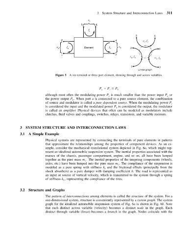
Figure 5 A six-terminal or three-port element, showing through and across variables.

P P P b
a
c
although most often the modulating power P is much smaller than the power input P or
a
c
the power output P . When port a is connected to a pure source element, the combination
b
of source and modulator is called a pure dependent source. When the modulating power P c
is considered the input and the modulated power P is considered the output, the modulator
b
is called an amplifier. Physical devices that often can be modeled as modulators include
clutches, fluid valves and couplings, switches, relays, transistors, and variable resistors.
3 SYSTEM STRUCTURE AND INTERCONNECTION LAWS
3.1 A Simple Example
Physical systems are represented by connecting the terminals of pure elements in patterns
that approximate the relationships among the properties of component devices. As an ex-
ample, consider the mechanical–translational system depicted in Fig. 6a, which might rep-
resent an idealized automobile suspension system. The inertial properties associated with the
masses of the chassis, passenger compartment, engine, and so on, all have been lumped
together as the pure mass m . The inertial properties of the unsprung components (wheels,
1
axles, etc.) have been lumped into the pure mass m . The compliance of the suspension is
2
modeled as a pure spring with stiffness k and the frictional effects (principally from the
1
shock absorbers) as a pure damper with damping coefficient b. The road is represented as
an input or source of vertical velocity, which is transmitted to the system through a spring
of stiffness k , representing the compliance of the tires.
2
3.2 Structure and Graphs
The pattern of interconnections among elements is called the structure of the system. For a
one-dimensional system, structure is conveniently represented by a system graph. The system
graph for the idealized automobile suspension system of Fig. 6a is shown in Fig. 6b. Note
that each distinct across variable (velocity) becomes a distinct node in the graph. Each
distinct through variable (force) becomes a branch in the graph. Nodes coincide with the