Page 490 - Mechanical Engineers' Handbook (Volume 2)

6 Stability 481

6.2 Polar Plots
The frequency response of a system described by a transfer function G(s) is given by
y (t) X G(j ) sin[ t G(j )]
/
1
ss
where X sin t is the forcing input and y (t) is the steady-state output. A great deal of
ss
information about the dynamic response of the system can be obtained from a knowledge
of G( j ). The complex quantity G( j ) is typically characterized by its frequency-dependent
magnitude G( j ) and the phase G( j ). There are many different ways in which this
/
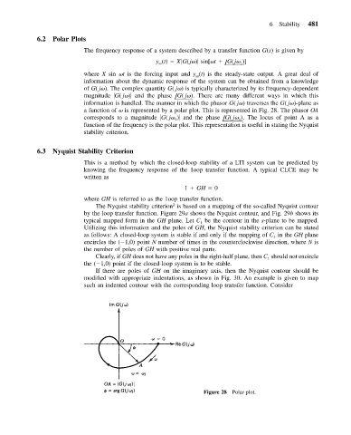
information is handled. The manner in which the phasor G( j ) traverses the G( j )-plane as
a function of is represented by a polar plot. This is represented in Fig. 28. The phasor OA
/
corresponds to a magnitude G( j ) and the phase G( j ). The locus of point A as a
1
1
function of the frequency is the polar plot. This representation is useful in stating the Nyquist
stability criterion.
6.3 Nyquist Stability Criterion
This is a method by which the closed-loop stability of a LTI system can be predicted by
knowing the frequency response of the 1oop transfer function. A typical CLCE may be
written as

1 GH 0
where GH is referred to as the 1oop transfer function.
2
The Nyquist stability criterion is based on a mapping of the so-called Nyquist contour
by the loop transfer function. Figure 29a shows the Nyquist contour, and Fig. 29b shows its
typical mapped form in the GH plane. Let C be the contour in the s-plane to be mapped.
1
Utilizing this information and the poles of GH, the Nyquist stability criterion can be stated
as follows: A closed-loop system is stable if and only if the mapping of C in the GH plane
1
encircles the ( 1,0) point N number of times in the counterclockwise direction, where N is
the number of poles of GH with positive real parts.
Clearly, if GH does not have any poles in the right-half plane, then C should not encircle
1
the ( 1,0) point if the closed-loop system is to be stable.
If there are poles of GH on the imaginary axis, then the Nyquist contour should be
modified with appropriate indentations, as shown in Fig. 30. An example is given to map
such an indented contour with the corresponding loop transfer function. Consider

Figure 28 Polar plot.