Page 492 - Mechanical Engineers' Handbook (Volume 2)

7 Steady-State Performance and System Type 483

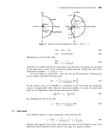
Figure 31 Nyquist contour and mapping for GH(s) K/s( s 1).

E(s) R(s) Y(s) (80)
Y(s) G (s)G (s)E(s) (81)
p
c
Substituting Eq. (81) in (80) yields
E(s) 1
(82)
R(s) 1 G (s)G (s)
p
c
called the error transfer function. It is important to note that the error dynamics are described
by the same poles as those of the closed-loop transfer function. Namely, the roots of the
characteristic equation 1 G (s)G (s) 0.
p
c
Given any input r(t) with L[r(t)] R(s), the error can be analyzed by considering the
inverse Laplace transform of E(s) given by
e(t) L 1 R(s)
1
1 G (s)G (s) (83)
c p
For the system’s error to be bounded, it is important to first assure that the closed-loop
system is asymptotically stable. Once the closed-loop stability is assured, the steady-state
error can be computed by using the final-value theorem. Hence
lim e(t) e lim sE(s) (84)
ss
t→ s→0
By substituting for E(s) in Eq. (84)
1
e lim s R(s) (85)
ss
s→0 1 G (s)G (s)
c
p
7.1 Step Input
If the reference input is a step of magnitude c, then from Eq. (85)
1 c c
e lim s (86)
ss
s→0 1 G (s)G (s) s 1 GG (0)
p
c
c
p
Equation (86) suggests that to have small steady-state error, the low-frequency gain of the
open-loop transfer function G G (0) must be very large. It is typical to define
c
p