Page 505 - Mechanical Engineers' Handbook (Volume 2)

496 Closed-Loop Control System Analysis

Figure 43 Quarter-square multiplier. Figure 44 Division.

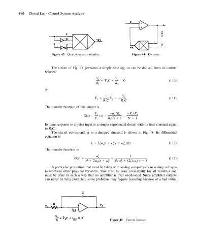
The circuit of Fig. 47 generates a simple time lag, as can be derived from its current
balance:
V 1 VC V 2 0 (110)
˙
R 1 2 R 2
or
1 V
˙
V V 1 (111)
2
RC 2 RC
1
2
The transfer function of this circuit is
V R /R R /R
G(s) 2 (s) 2 1 2 1
V 1 R Cs 1 s 1
2
Its time response to a pulse input is a simple exponential decay, with its time constant equal
to R C.
2
The circuit corresponding to a damped sinusoid is shown in Fig. 48. Its differential
equation is
2
2
¨ y 2 ˙y y ƒ(t) (112)
n
n
n
The transfer function is
2 1
G(s) n (113)
2
2
s 2 s 2 n s / (2 / ) s 1
2
n
n
n
A particular precaution that must be taken with analog computers is in scaling voltages
to represent other physical variables. This must be done consistently for all variables and
must be done in such a way that no amplifier is ever overloaded. Since amplifier outputs
can never be fully predicted, some problems may require rescaling because of a bad initial

Figure 45 Current balance.