Page 517 - Mechanical Engineers' Handbook (Volume 2)

508 Control System Performance Modification

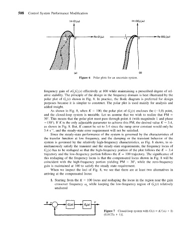
Figure 6 Polar plots for an uncertain system.

frequency gain of sG G (s) effectively at 100 while maintaining a prescribed degree of rel-
c
p
ative stability. The principle of the design in the frequency domain is best illustrated by the
polar plot of G (s) shown in Fig. 8. In practice, the Bode diagram is preferred for design
p
purposes because it is simpler to construct. The polar plot is used mainly for analysis and
added insight.
As shown in Fig. 8, when K 100, the polar plot of G (s) encloses the ( 1,0) point,
p
and the closed-loop system is unstable. Let us assume that we wish to realize that PM
30 . This means that the polar plot must pass through point A (with magnitude 1 and phase
150 ). If K is the only adjustable parameter to achieve this PM, the desired value K 3.4,
as shown in Fig. 8. But, K cannot be set to 3.4 since the ramp error constant would only be
3.4 s , and the steady-state error requirement will not be satisfied.
1
Since the steady-state performance of the system is governed by the characteristics of
the transfer function at low frequency, and the damping or the transient behavior of the
system is governed by the relatively high-frequency characteristics, as Fig. 8 shows, to si-
multaneously satisfy the transient and the steady-state requirements, the frequency locus of
G (s) has to be reshaped so that the high-frequency portion of the plot follows the K 3.4
p
trajectory and the low-frequency portion follows the K 100 trajectory. The significance of
this reshaping of the frequency locus is that the compensated locus shown in Fig. 8 will be
coincident with the high-frequency portion yielding PM 30 , while the zero-frequency
gain is maintained at 100 to satisfy the steady state requirement.
When we inspect the loci of Fig. 8, we see that there are at least two alternatives in
arriving at the compensated locus:
1. Starting from the K 100 locus and reshaping the locus in the region near the gain
crossover frequency while keeping the low-frequency region of G (s) relatively
p
g
unaltered

Figure 7 Closed-loop system with G(s) K/[s(s 1)
(0.0125s 1)].