Page 518 - Mechanical Engineers' Handbook (Volume 2)

3 Hall Chart 509

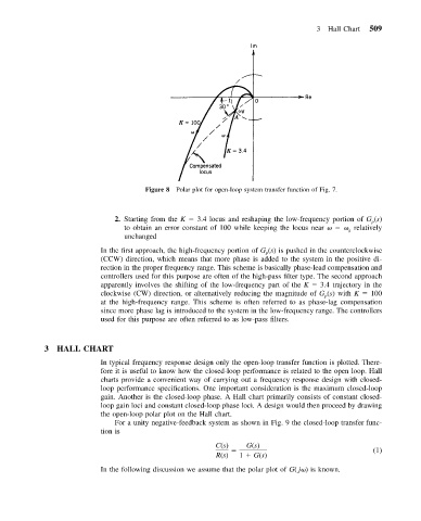
Figure 8 Polar plot for open-loop system transfer function of Fig. 7.

2. Starting from the K 3.4 locus and reshaping the low-frequency portion of G (s)
p
to obtain an error constant of 100 while keeping the locus near relatively
g
unchanged
In the first approach, the high-frequency portion of G (s) is pushed in the counterclockwise
p
(CCW) direction, which means that more phase is added to the system in the positive di-
rection in the proper frequency range. This scheme is basically phase-lead compensation and
controllers used for this purpose are often of the high-pass filter type. The second approach
apparently involves the shifting of the low-frequency part of the K 3.4 trajectory in the
clockwise (CW) direction, or alternatively reducing the magnitude of G (s) with K 100
p
at the high-frequency range. This scheme is often referred to as phase-lag compensation
since more phase lag is introduced to the system in the low-frequency range. The controllers
used for this purpose are often referred to as low-pass filters.

3 HALL CHART
In typical frequency response design only the open-loop transfer function is plotted. There-
fore it is useful to know how the closed-loop performance is related to the open loop. Hall
charts provide a convenient way of carrying out a frequency response design with closed-
loop performance specifications. One important consideration is the maximum closed-loop
gain. Another is the closed-loop phase. A Hall chart primarily consists of constant closed-
loop gain loci and constant closed-loop phase loci. A design would then proceed by drawing
the open-loop polar plot on the Hall chart.
For a unity negative-feedback system as shown in Fig. 9 the closed-loop transfer func-
tion is

C(s) G(s)
(1)
R(s) 1 G(s)
In the following discussion we assume that the polar plot of G( j ) is known.