Page 528 - Mechanical Engineers' Handbook (Volume 2)

5 Root Locus 519

b. The n m asymptote angles are given by
180 N

N
n m
where N takes on values 1, 3, 5, 7,....For each N, two angles are computed and the
procedure is repeated until n m angles are obtained.
Rule 5. If to the right of a point on the real axis there lies an odd number of open-loop
poles and zeros, then it is a point on the root loci.
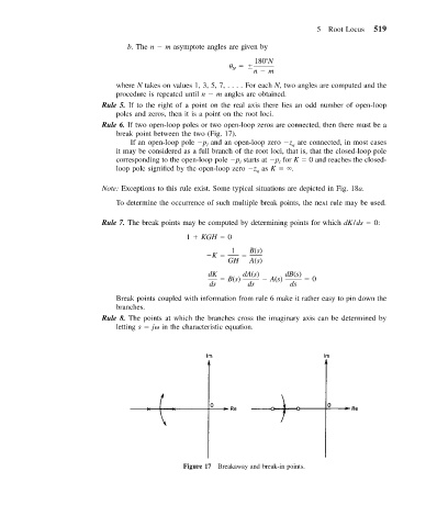
Rule 6. If two open-loop poles or two open-loop zeros are connected, then there must be a
break point between the two (Fig. 17).
If an open-loop pole p and an open-loop zero z are connected, in most cases
l
q
it may be considered as a full branch of the root loci, that is, that the closed-loop pole
corresponding to the open-loop pole p starts at p for K 0 and reaches the closed-
l
l
loop pole signified by the open-loop zero z as K .
q
Note: Exceptions to this rule exist. Some typical situations are depicted in Fig. 18a.
To determine the occurrence of such multiple break points, the next rule may be used.

Rule 7. The break points may be computed by determining points for which dK/ds 0:
1 KGH 0
1 B(s)
K
GH A(s)
dK dA(s) dB(s)
B(s) A(s) 0
ds ds ds
Break points coupled with information from rule 6 make it rather easy to pin down the
branches.
Rule 8. The points at which the branches cross the imaginary axis can be determined by
letting s j in the characteristic equation.

Figure 17 Breakaway and break-in points.